Project 4: Image Warping and Mosaicing

Recovering the Homographies

A homography is given by a transformation sending $v_{1} = \begin{bmatrix} x \\ y \\ 1 \end{bmatrix}$ to $v_{2} = \begin{bmatrix} x^{\prime} \\ y^{\prime} \\ 1 \end{bmatrix}$ mod scaling through a matrix:

\begin{equation*} c \begin{bmatrix} x^{\prime} \\ y^{\prime} \\ 1 \end{bmatrix} = \begin{bmatrix} h_{1} & h_{2} & h_{3} \\ h_{4} & h_{5} & h_{6} \\ h_{7} & h_{8} & 1 \end{bmatrix} \begin{bmatrix} x \\ y \\ 1 \end{bmatrix} \end{equation*}

Multiplying everything out, we get:

\begin{align*} cx^{\prime} &= h_{1}x + h_{2}y + h_{3} \\ cy^{\prime} &= h_{4}x + h_{5}y + h_{6} \\ c &= h_{7}x + h_{8}y + 1 \end{align*}

and substituting:

\begin{align*} (h_{7}x + h_{8}y + 1)x^{\prime} &= h_{1}x + h_{2}y + h_{3} \\ (h_{7}x + h_{8}y + 1)y^{\prime} &= h_{4}x + h_{5}y + h_{6} \end{align*}

will give the system of equations:

\begin{align*} h_{1}x + h_{2}y + h_{3} + 0h_{4} + 0h_{5} + 0h_{6} - h_{7}xx^{\prime} - h_{8}yx^{\prime} - 1x^{\prime} &= 0 \\ 0h_{1} + 0h_{2} + 0h_{3} + h_{4}x + h_{5}y + h_{6} - h_{7}xy^{\prime} - h_{8}yy^{\prime} - 1y^{\prime} &= 0 \end{align*}

This gives a way to solve for the entries of the matrix $H$ through a different linear equation $Ax = b$ where $A$ is a $2 \times 8$ matrix, $x$ is the vector containing the entries $h_1, \ldots, h_8$, and $b$ is the vector containing the values $x', y'$. This is extendable to include more points in our homography mapping and can be solved through least squares to find the projective mapping

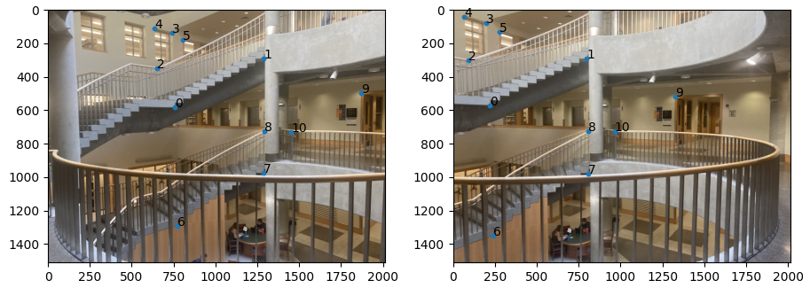
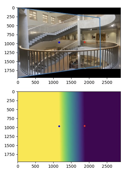
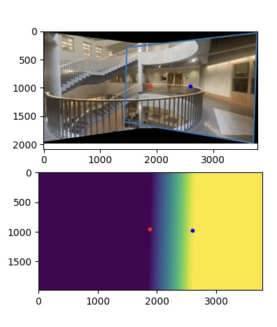
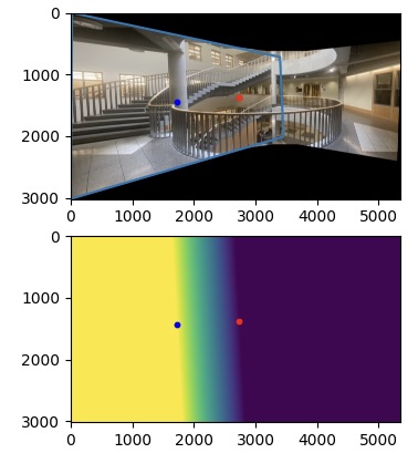
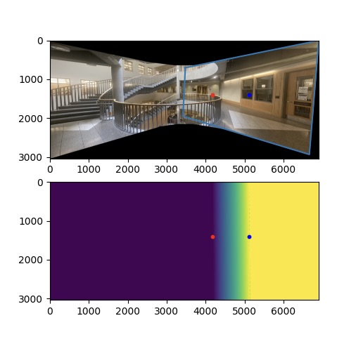
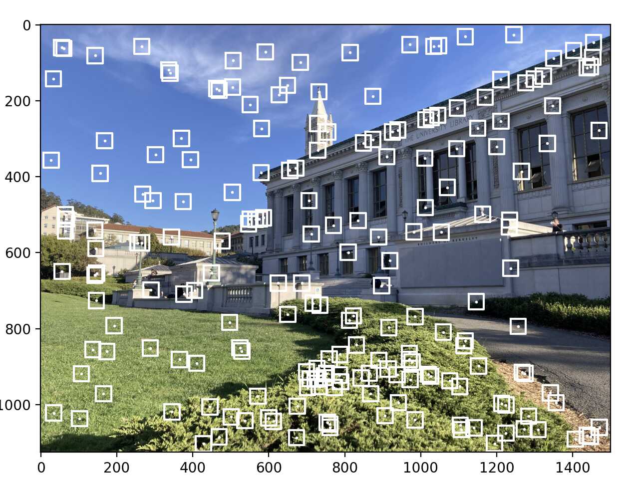
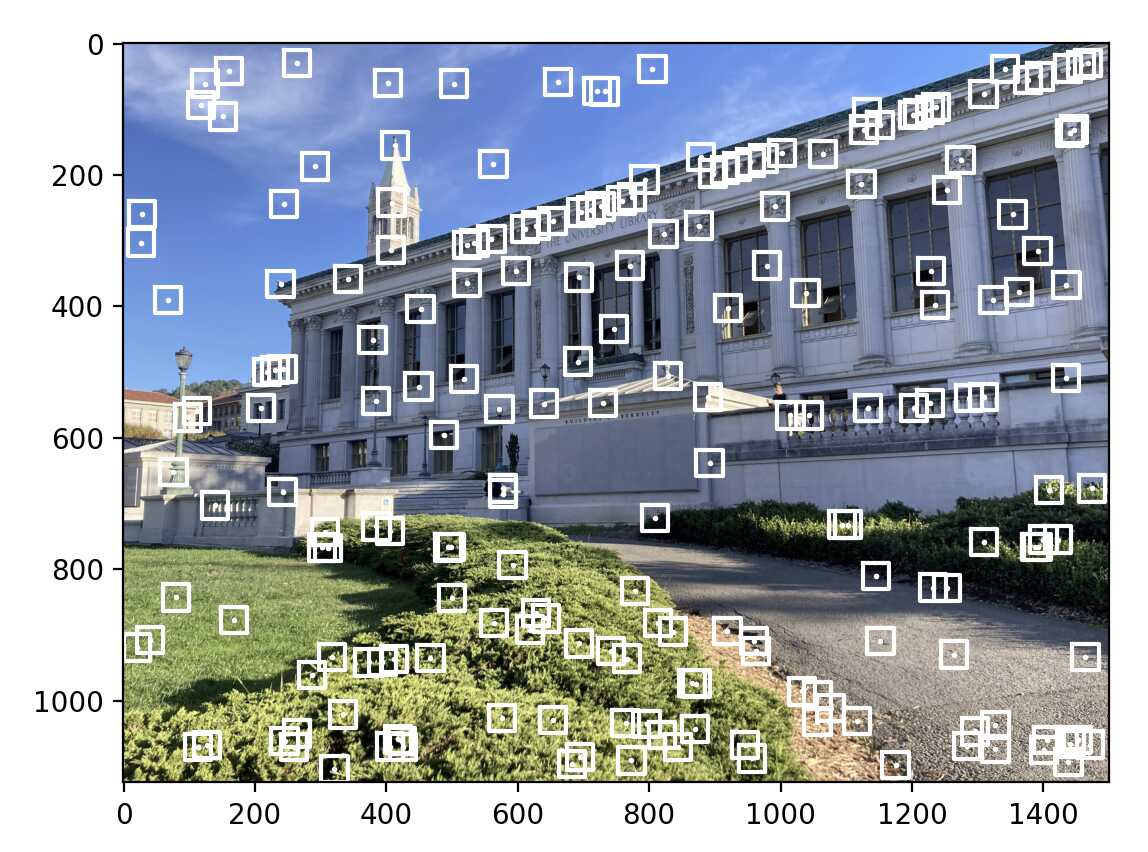
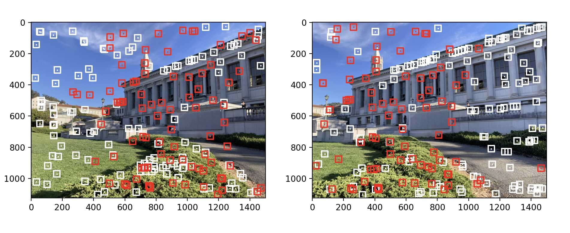
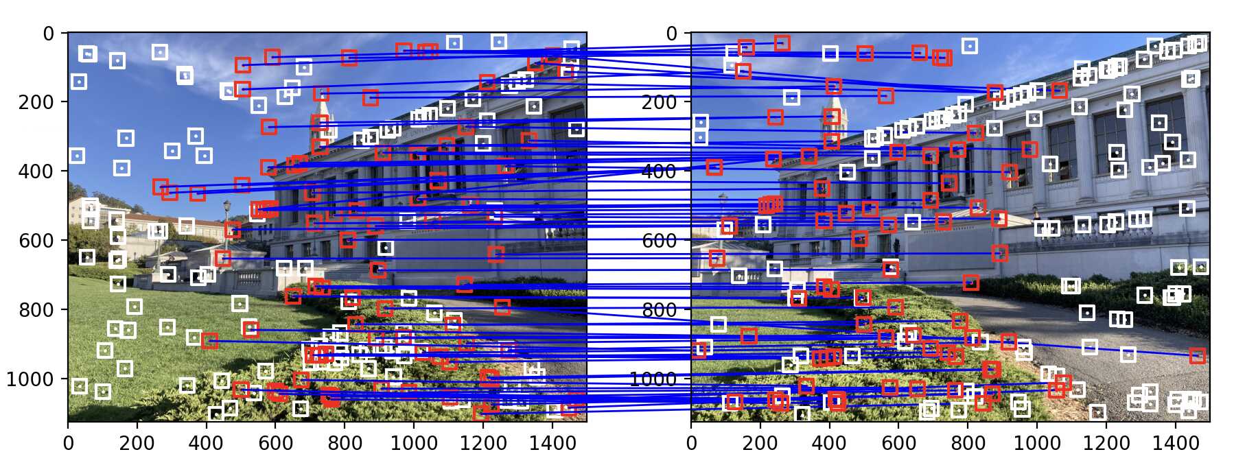
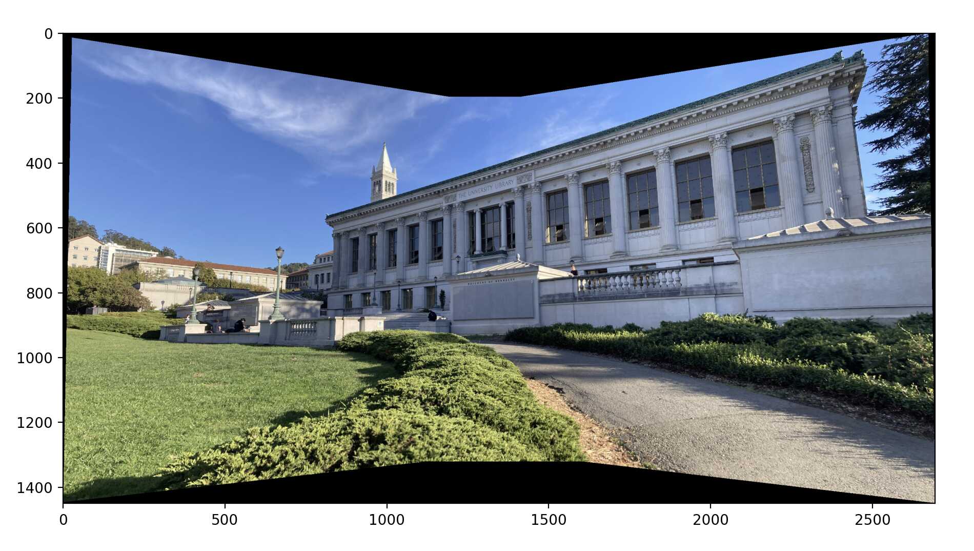
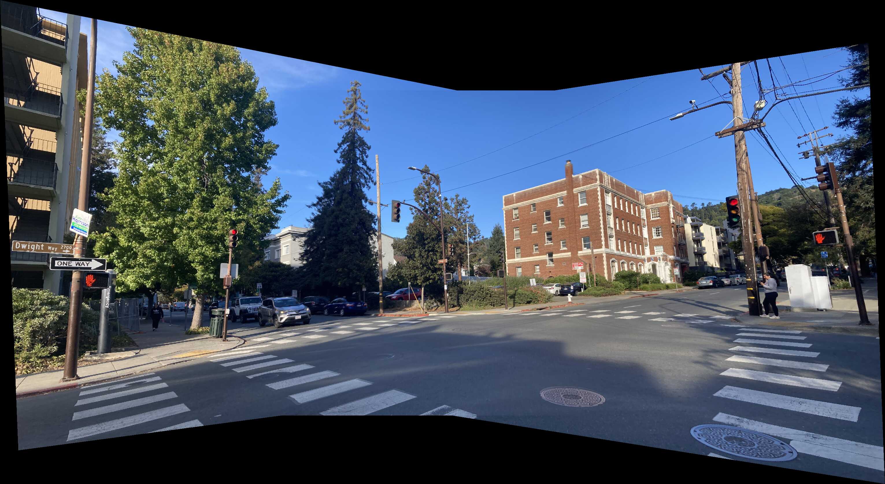
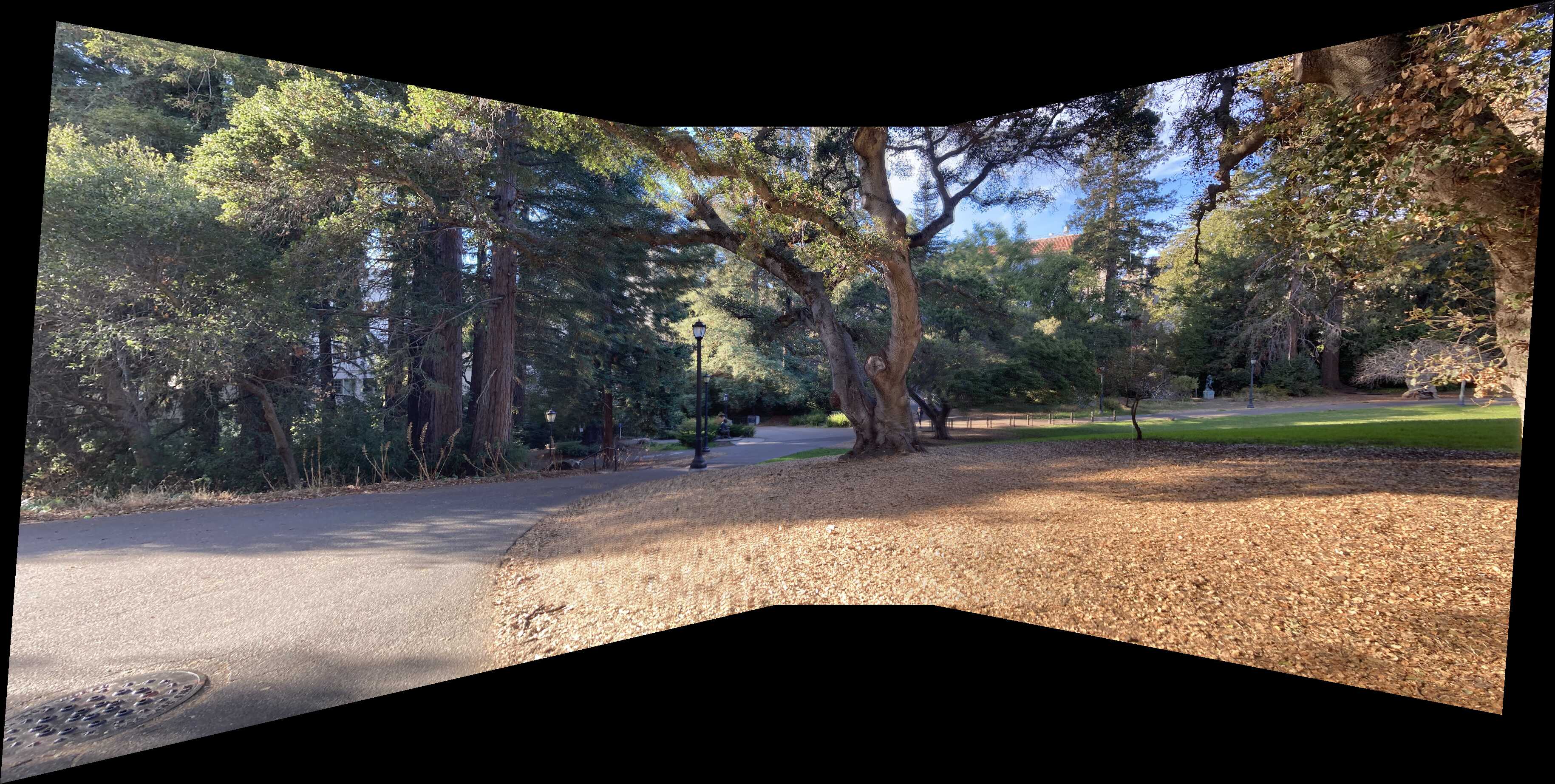
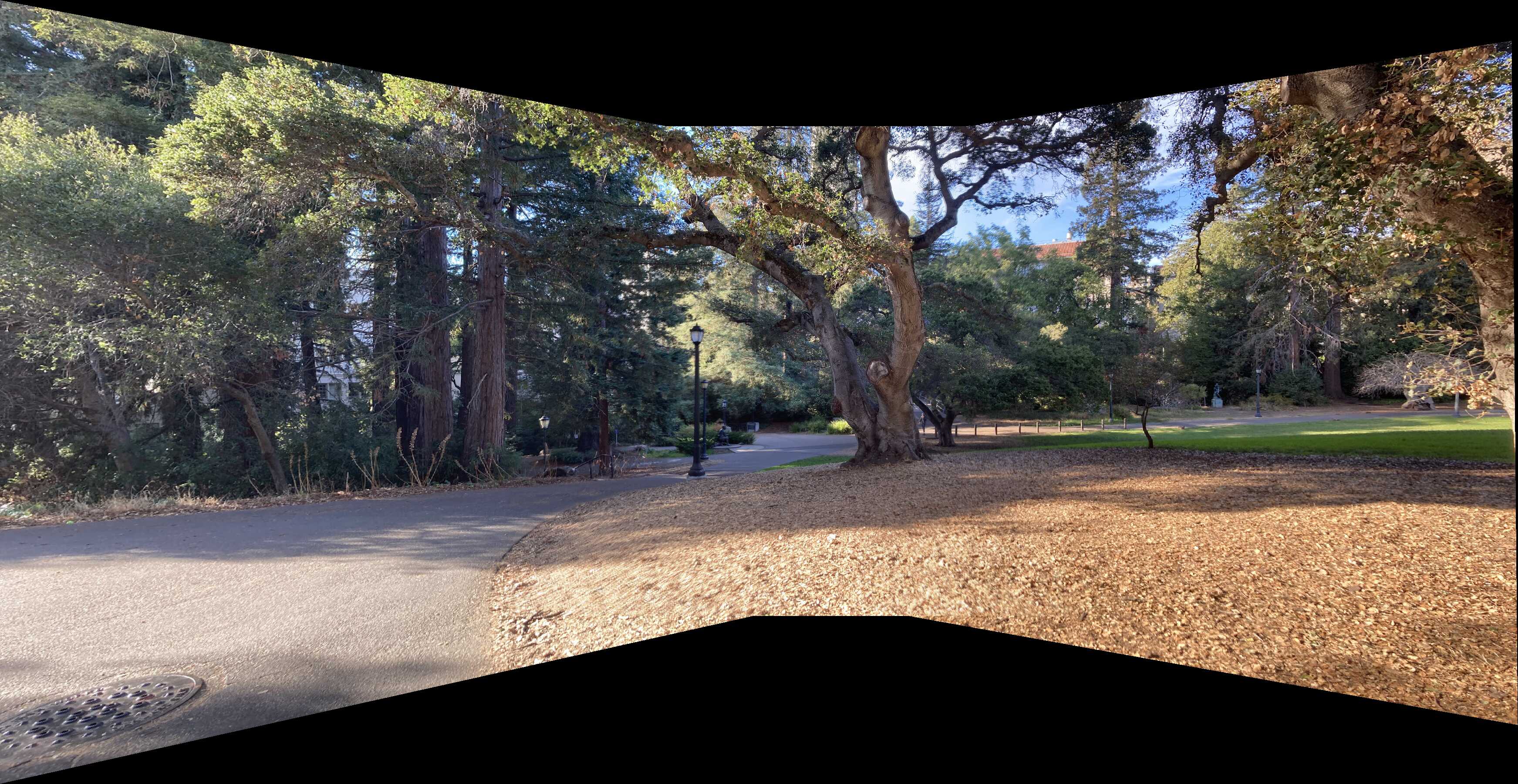
Here is an example of the point correspondences that I used to compute the homography

Warping the Image

This process was very similar to the last project, but instead, the warp would be determined by four corners under the homography transformation. After calculating the new corners, a resulting image would be set to encompass the warped image. The pixel values in the new image $B$ would be determined by where the pixel landed under the transformation $H^{-1}$.

Since the pixel location under $H^{-1}$ is not exact, I used griddata to interpolate for the pixel value using the location and values in the original image as the data. Here is the result of the warp on the left and the base image of the panorama on the right

Rectification

One interesting application of image warping by homography is to emulate a snapshot of the image from a different perspective. In changing the camera angle via homography, we attempt to capture the pixels outside the image, and therefore, the image is shifted further to the peripheral making it seem distorted. This is why rectification will work well when dealing with small shifts in the perspective. Here are some examples that I ran my code on:

Image Mosaic

The first step is to correctly align the images. Here I used zero padding:

The images cannot be directly added together and averaged at the intersection because there is different lighting and exposure across images. To fix this, I created a set of two images. Let the image on the left be image $A$ and the image on the right be image $B$. In one image, image $A$ would dominate, meaning that on $\text{image}(A) \cap \text{image} B$, I would set the pixel values to be that of image $A$. The other case would be an image where image $B$ dominates. Here is an example of creating these images:

Then for the blending, notice that image $A$ captures the scene more accurately the closer the pixels are to the center of image $A$. The same goes for image $B$. So to get a blend, a linear interpolation between their centers can be calculated (through griddata) and put into a mask. The output image is given by \begin{equation*} \text{mosaic} = \text{mask} \cdot \text{dominantA} + (1 - \text{mask}) \cdot \text{dominantB} \end{equation*} Here is an iterative approach to the blending:

Although it is possible to separate the frequencies into high and low frequencies, blending the lower frequencies and choosing one of the higher frequencies, I had more success just directly blending the images. This is because a small misalignment of about 5 pixels can cause the high frequencies in one image to look discontinuous with the high frequencies in the other. This caused the railing to look cutoff at certain areas in my previous blends. Here is the final result without separating the frequencies:

Detecting Corner Features

The Harris corner detector defines a corner centered on pixel $u, v$ on some window of size $w$ if for any shift in $x$ or $y$, the squared difference between the shifted window and the original is non-zero.

We notice that when the red window is over a monocolor surface, shifts of the window in either the $x$ or $y$ direction results in no change in what the window sees. For the line example, the window only sees a change when we move in the vertical direction. When the window is shifted in a horizontal direction, the difference is $0$. This would be defined as an edge. Finally, we have the vertex of a triangle. In this case, any change in either the $x$ or $y$ direction results in a change in what the window sees. We can also plot the squared difference as a function over displacement of the window at a pixel. Here's what it would look like for the above examples:

The first one is circular because at the origin, displacement is $(0, 0)$, and as we have more displacement, the error increases between the original and the displaced window. The second one is like a valley because along the horizontal direction, displacement does not change what the window sees, so the error is $0$. As we move in the vertical direction, the error increase. Finally, if the window is over a monocolor surface, the error will be $0$.
Implementation of finding the harris corners and corner strength was given as starter code. Also, I was not able to plot all harris corners because there were too many detected, and it would completely blanket the image. A view of some of the filtered out corners will be shown in the next section.

Extracting Feature Descriptors

Feature descriptors describe what is happening locally at a pixel. They usually small $8 \times 8$ pixels, and can be used to match features across images. This is done by the squared difference between the descriptors. At the original resolution, however, the descriptors are not robust to small errors such as differences in orientation and perspective. To fix this, a $40 \times 40$ window is sampled around the pixel, convolved with a Gaussian kernel, and downsampled by $5$. The descriptor is finally normalized to make it resilient to differences in luminence:

And here are all the feature descriptors extracted from the images:

Feature Matching

Notice that in the previous picture, some feature descriptors in one image are not present in the other. So we need a way to throw away feature descriptors as well as match the remaining feature descriptors. One problem with finding the nearest neighbor from one image to another by squared error is that two descriptors could yield a small error, but the probability of it being an incorrect match shares significant overlap with the probability that it is a correct match:

This is seen on the left where a nearest neighbor squared error of $10$ will not be a strong indicator of whether the pair is a correct match or not. One instance in which this might be a problem is if the descriptors are not present in both images. In the case that the descriptor from one image matches with the descriptor in the other, we have an outlier match, which will throw off the key point matching.

In contrast, we can instead look at the ratio between the closest match and the second closest match error. This gives a much better separation between the probability density of correct matches vs incorrect matches. The algorithm is reduce to setting the threshold. If the ratio of the error is high, then we can reject both descriptors as being a part of the final match. If the ratio is low, then we have found a match between the descriptor and its nearest neighbor.

Here, the white feature descriptors are from before feature matching. The red is after feature matching. Notice that the feature descriptors that are preserved tend to be on the overlap region of the two images.

Robust Homography

All that is left is to produce the homography. One problem we have is that many of the feature descriptors do not represent a true match. For example, in the right image below, there is a red feature descriptor in the bottom right corner, which clearly lies outside of the image on the left. To make the homography robust to incorrect matches, we can use the RANSAC method.

RANSAC is a statistical algorithm which, for a chosen set of data, finds the inliers and outliers given our distribution. In our example, given four points which define a homography, we want to see how likely the homography on these points is to be the true homography. To do this, we compute the homography on the four points, and for every other point in the same image, we apply the homography. We then see if its matching feature descriptor lie within half a pixel of each other. If they do, then we classify them as an inlier, meaning they agree with the homography, otherwise, they are an outlier. The problem then reduces to choosing the homography that maximizes the number of inliers.

A Comparison

Here are the results of the homography done manually vs automatically. The image on top will be the one doe manually and the one below is automatic. There is a noticeable trend that the automatic alignment and robust homography tends to do better in areas that have lots of trees. In the examples below, my manual alignment tends to result in the leaves being blurred, while the automatic alignment is much more consistent in aligning the leaves.

Near Anthropology

Street Intersection

Faculty Glade