Fun With Diffusion Models!

Forward Process

In the forward process, an image is denoised by subtracting away the noise that is predicted to be in the image. For diffusion, the model is trained on the noise given by: \begin{equation*} \mathcal{N}(0, \sqrt{1 - \overline{\alpha}}) \end{equation*} Adding this noise to our base image \begin{equation*} \sqrt{\overline{\alpha}} \cdot x_0 \end{equation*} gives the noisy image that the network sees at $\alpha$, the interpolation factor. Here, $\alpha$ is determined by a schedule, and we obtain it by $\alpha[t]$ where $t$ is the timestep $t \in [0, 999]$. Here are some results of generating the noisy image:

Denoising

Classic Denoising

In classic denoising, we attempt to hide irregularities in the image through some averaging/smoothing filter such as the gaussian filter. By pulling data from neighboring pixels, we can decrease the impact of noise on the image. This does well when there is little noise, but fails at high noise levels, which is seen in all three attempts.

Campanile Clean t250 — Denoise $t = 250$

Campanile Clean t500 — Denoise $t = 500$

Campanile Clean t750 — Denoise $t = 750$

One-Step Denoising

In one step denoising, we feed in the noisy image and the current timestep, and the model recovers the amount of noise that is predicted to be in the image. Recall that we used the equation: \begin{equation*} x_{t} = \sqrt{\overline{\alpha}} \cdot x_{0} + \sqrt{1 - \overline{\alpha}} \cdot \epsilon \end{equation*} for the forward process. So we can recover the original image $x_0$ by: \begin{equation*} x_{0} = \dfrac{x_{t} - \sqrt{1 - \overline{\alpha}} \cdot \epsilon}{\sqrt{\overline{\alpha}}} \end{equation*}

This does much better than the low-pass filter, but the image is till blurry compared to the original. For example, the trees have lost their texture and takes on a flat green texture.

Iterative Denoising

In iterative denoising, rather than subtracting all noise out in one step, we subtract a little bit of noise over many steps and repredict the next amount of noise. The process is sped up by taking strided timesteps and the new formula is given by: \begin{equation*} x_{t^{\prime}} = \dfrac{\sqrt{\overline{\alpha_{t^{\prime}}}}\beta_{t}}{1 - \overline{\alpha}_{t}}x_{0} + \dfrac{\sqrt{\alpha_{t}}(1 - \overline{\alpha}_{t^{\prime}})}{1 - \overline{\alpha_{t}}}x_{t} + v_{\sigma}\end{equation*} The values are given by:

$x_{t}$ is the noisy image at time $t$
$x_{t^{\prime}}$ is the noisy image at the next timestep
$\overline{\alpha}_{t}$ is $\alpha[t]$
$\alpha_{t} = \frac{\overline{\alpha}_{t}}{\overline{\alpha_{t^{\prime}}}}$
$\beta_{t} = 1 - \alpha_{t}$
$x_{0}$ is the predicted clean image given by the one step formula

Campanile Iterative Denoise 1 — $t = 690$

Campanile Iterative Denoise 2 — $t = 540$

Campanile Iterative Denoise 3 — $t = 390$

Campanile Iterative Denoise 4 — $t = 240$

Campanile Iterative Denoise 5 — $t = 90$

The resulting image looks sharper than the previous ones

A Comparison

It is noticeable that gaussian denoising is not very effective when there is too much noise. So we have to go for nonlinear denoising methods, such as one step and iterative denoising.

Diffusion Model Sampling

We can also denoise pure noise, rather than starting from a noisy image. Here are $5$ results:

Classifier Free Guidance

In CFG, the model uses conditional classification. We can generate two noise predictions off of our current image $\epsilon_{c}, \epsilon_{u}$ such that our new predicted noise is: \begin{equation*} \epsilon = (1 - \gamma)\epsilon_{u} + \gamma \epsilon_{c} \end{equation*} This means that when $\gamma > 1$ the noise prediction leans more towards using the conditional noise. From the small update the images become much more recognizable:

Image to Image Translation

Rather than starting with random noise, we can start with a noisy base image and run iterative cfg to get variations from our base image. This is done by running the forward noising process and running the previous algorithm on the noisy image.

Editing Hand-Drawn/Web Images

We can also denoise hand-drawn and web images:

Inpainting

We can also inpaint an image given the work done so far. Rather than subtracting out the noise calculated at each step from our entire image, we only subtract out the calculated noise in a section of our image. This means that for all noise outside the area we want to inpaint, we replace it with the original image processed through the forward noising function.

Text Conditional Image to Image Translation

Rather than keeping the prompt set to "a high quality photo", we can replace it with a text prompt from the prompt embedding. This means that rather than denoising unconditionally, we denoise based on the prompt given, which will give the image a push towards what is specified by the prompt.

Campanile Translation Rocket t_1 — $t = 1$

Campanile Translation Rocket t_1 gif — $t = 1$

Campanile Translation Rocket t_2 — $t = 3$

Campanile Translation Rocket t_2 gif — $t = 3$

Campanile Translation Rocket t_3 — $t = 5$

Campanile Translation Rocket t_3 gif — $t = 5$

Campanile Translation Rocket t_4 — $t = 7$

Campanile Translation Rocket t_4 gif — $t = 7$

Campanile Translation Rocket t_5 — $t = 10$

Campanile Translation Rocket t_5 gif — $t = 10$

Campanile Translation Rocket t_6 — $t = 20$

Campanile Translation Rocket t_6 gif — $t = 20$

We see that the images look more similar to the base image (Campanile) when we start off with less noise, but still resembles a rocket, which was the prompt embed used.

Visual Anagrams

We can also flip the image at each step, denoise and flip it back to make a separate denoising step towards a different prompt embed. This allows us to make a flip illusion, where flipping the image reveals a hidden image. Hover over the images to visualize the result:

Flip Illusion Skull, Waterfall — A Waterfall

Flip Illusion Man, Campfire — A Campfire

Flip Illusion Man with Hat, Campfire — A Campfire

Flip Illusion Dog, Snow Mountain — A Snowy Village

Hybrid Images

A hybrid image is one where one subject in an image dominates when viewed up close and a different one dominates when viewed afar. We can again modify the noise added, this time taking the low frequencies of the predicted noise from one prompt embedding and adding it to the high frequencies of a different prompt embedding. Hover over the images to see the result:

Skull Snow Mountain hybrid — A Snow Mountain

Pencil Snow Mountain hybrid — A Snowy Village

Unconditional Unet

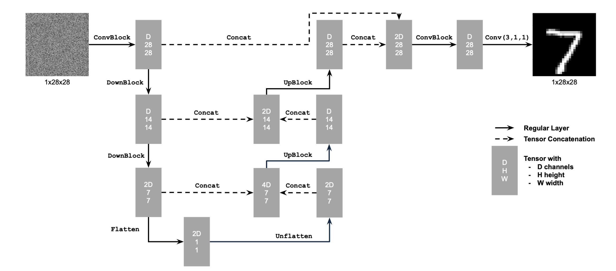
The unet is a convolutional network designed to output images from an input of a images. In the downward part of the net, we run the images through convolution and max pooling layers to increase the perception of the network. Going back up, we want to recover our image, so we add concatenations with information from our previous layers.

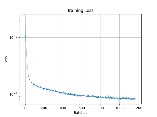
In a one step denoising process, we can use our unet to directly predict the clean image from a noisy input. To train the unconditional network, we fix the noise level to $\sigma = 0.5$ and noise an image by the given formula: \begin{equation*} x = x_{0} + \varepsilon \end{equation*} where \begin{equation*} \varepsilon \sim \mathcal{N}(0, \sigma^{2}) \end{equation*} We feed $x$ into the network and estimate the loss between $\hat{x}$ and $x_{0}$

Unconditional Unet Loss — After 5 epochs

Here are some results, where the clean image is on the left, the noisy image is on the middle, and the predicted image is on the right of each figure:

The unconditional unet does not do very well with higher noise levels, as there was no input on the amount of noise in our training. From left to right, the model was given images with noise levels of $0.0, 0.2, 0.4, 0.6, 0.8, $ and $1.0$

Various noise level denoisings — Epoch 1 Denoising

Conditional Unet

In a conditional unet, more information is given to the model and perform the denoising iteratively for better results. We define a new one step noising process: \begin{equation*} x_{t} = \sqrt{1 - \overline{\alpha_{t}}}x_{0} + \sqrt{\overline{\alpha_{t}}}\varepsilon \end{equation*} where \begin{equation*} \varepsilon \sim \mathcal{N}(0, I) \end{equation*} We want to predict the cleaner image given a noisy image and this is given by some function of $x_{t}, x_{0}$: \begin{equation*} p(x_{t - 1} \mid x_{t}) = \mathcal{N}(\mu_{t}(x_{t}, x_{0}), \tilde{\beta} I) \end{equation*} so \begin{equation*} x_{t - 1} = \dfrac{\sqrt{\overline{\alpha_{t - 1}}}\beta_{t}}{1 - \overline{\alpha_{t}}}x_{0} + \dfrac{\sqrt{\alpha_{t}}(1 - \overline{\alpha}_{t - 1})}{1 - \overline{\alpha}_{t}}x_{t} + \tilde{\beta}_{t}z, \, \tilde{\beta}_{t} = \dfrac{1 - \overline{\alpha}_{t - 1}}{1 - \overline{\alpha}_{t}}\beta_{t} \end{equation*} We define our $\beta_{t}$ as linear in $[0, 999]$, $\overline{\alpha}_{t} = 1 - \beta_{t}$ and $\alpha_{t} = \prod_{i = 0}^{t}\overline{\alpha}_{i}$. This gives us a way to recover a cleaner image $x_{t - 1}$ in terms of the predicted noise $\hat{\varepsilon}$ and $x_{t}$.

We first update the architecture by embedding the time and label of the training data. This is done by running both these through a linear layer, gelu, then another linear layer. We do this two times and embed at the unflatten layer and up convolve layer:

\begin{equation*} x = c \cdot x + t \end{equation*}

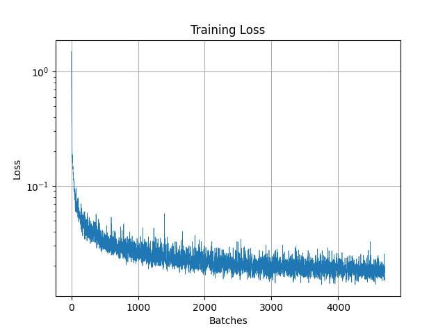
The forward process in the conditional unet is mostly the same. We add noise given by our new one step noising process. A mask is also created with a certain probability to run unconditioned predictions to make the model more flexible. Instead of predicting the clean image, the model will predict the noise and we update it based on $MSE(\hat{\varepsilon}, \varepsilon)$

In the sampling/denoising process, we iteratively predict the cleaner image given the formula for $x_{t - 1}$ calculated above. Hover over the images to see the denoising in action: