Project 1: The Rendering Pipeline

Drawing Triangles

Triangles are both simple and flexible making them important when it comes to drawing to the screen. The first method of drawing a triangle involves checking for each pixel, whether it lies inside or outside of the triangle we want to draw.

We do this through the half-plane point in polygon test. Given three points \(p_{1}, p_{2}, p_{3}\) oriented counter clockwise, we want to see if \(p\) lies inside the triangle. We can first compute the normals \(n_{1}, n_{2}, n_{3}\):

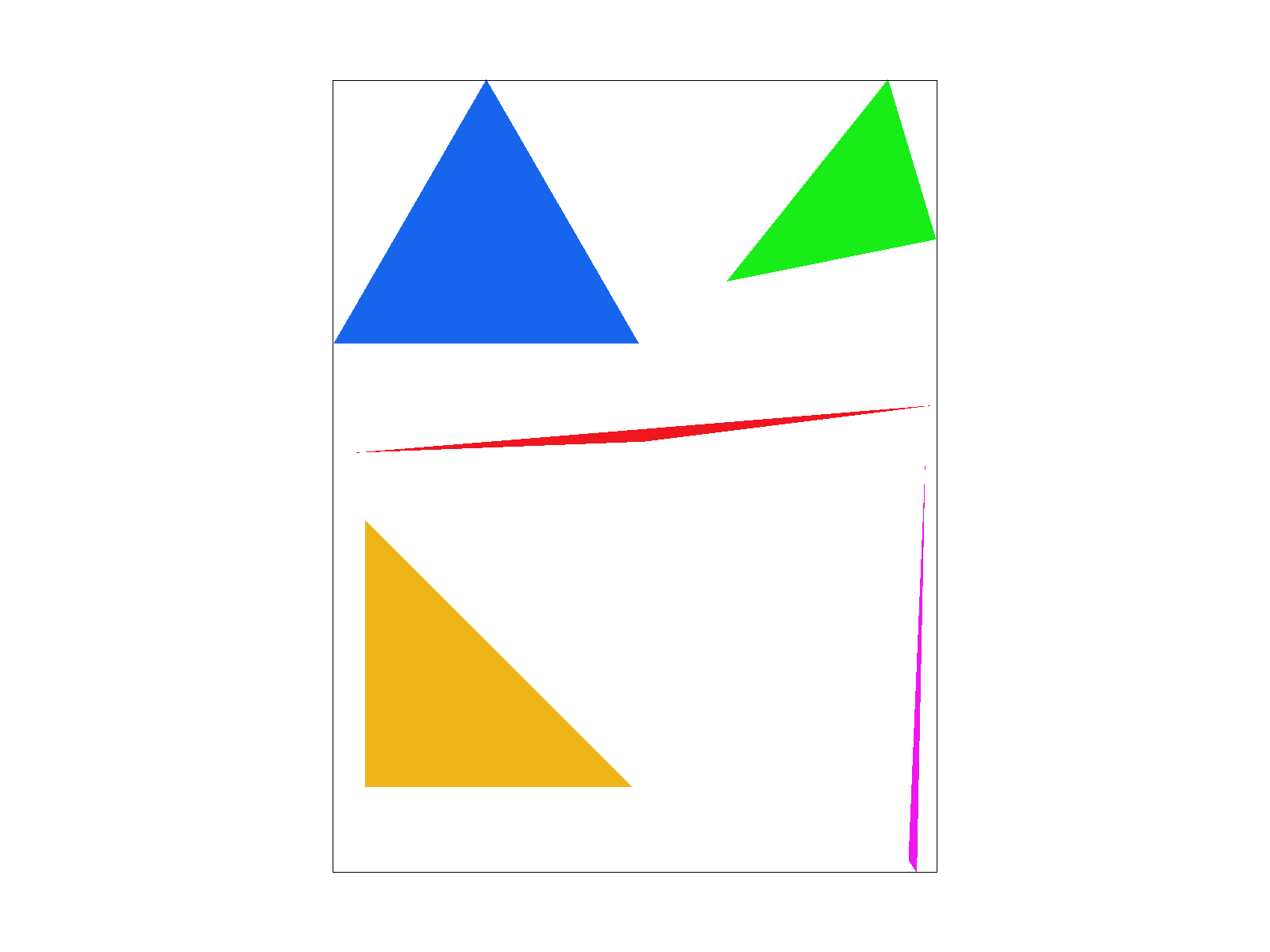
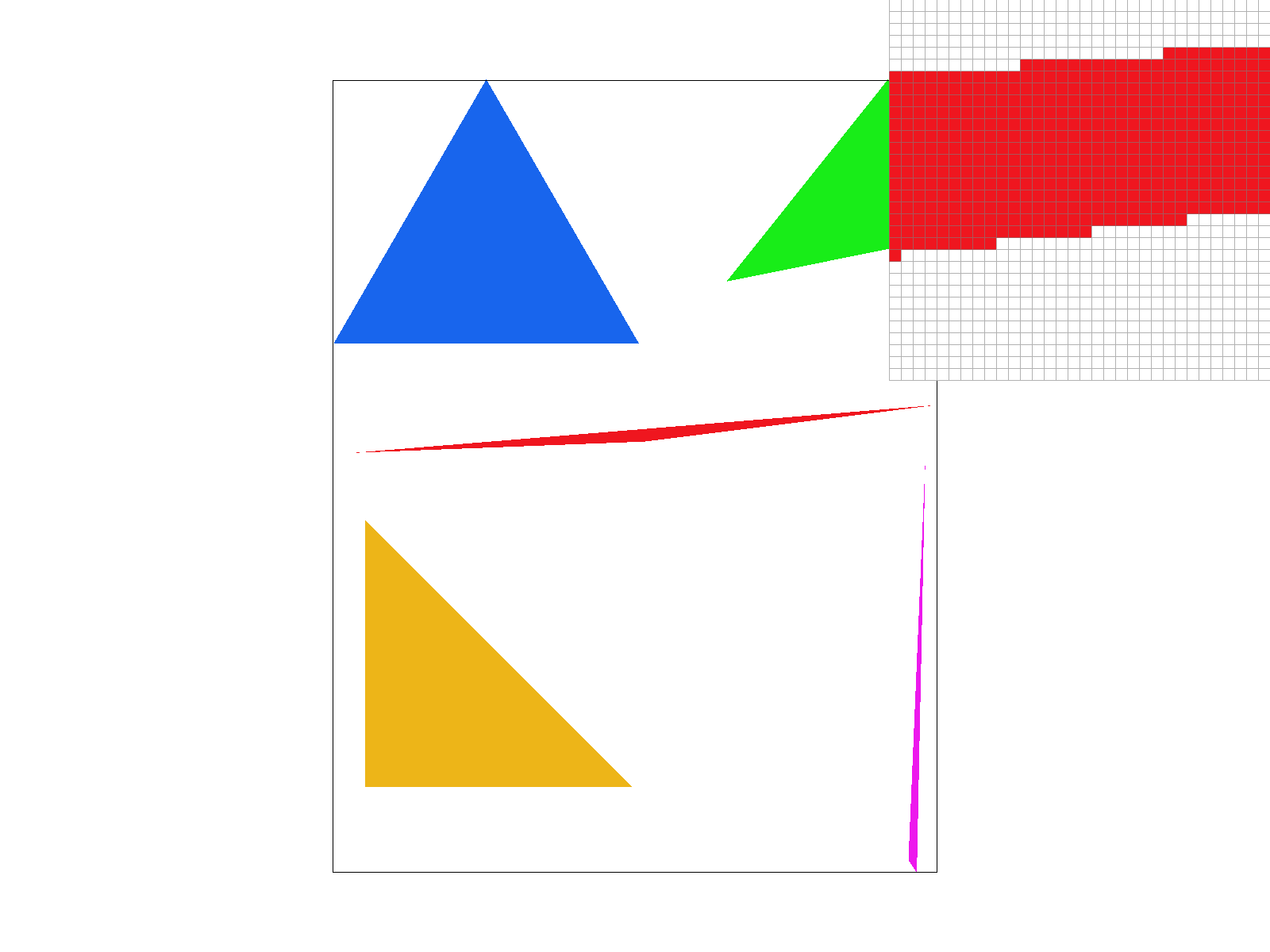
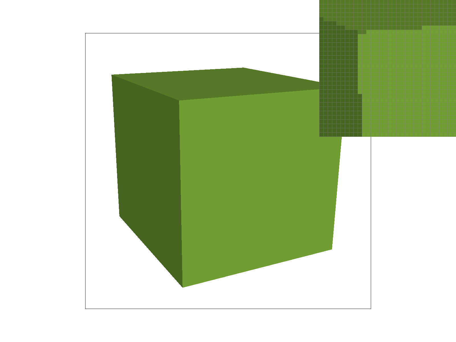
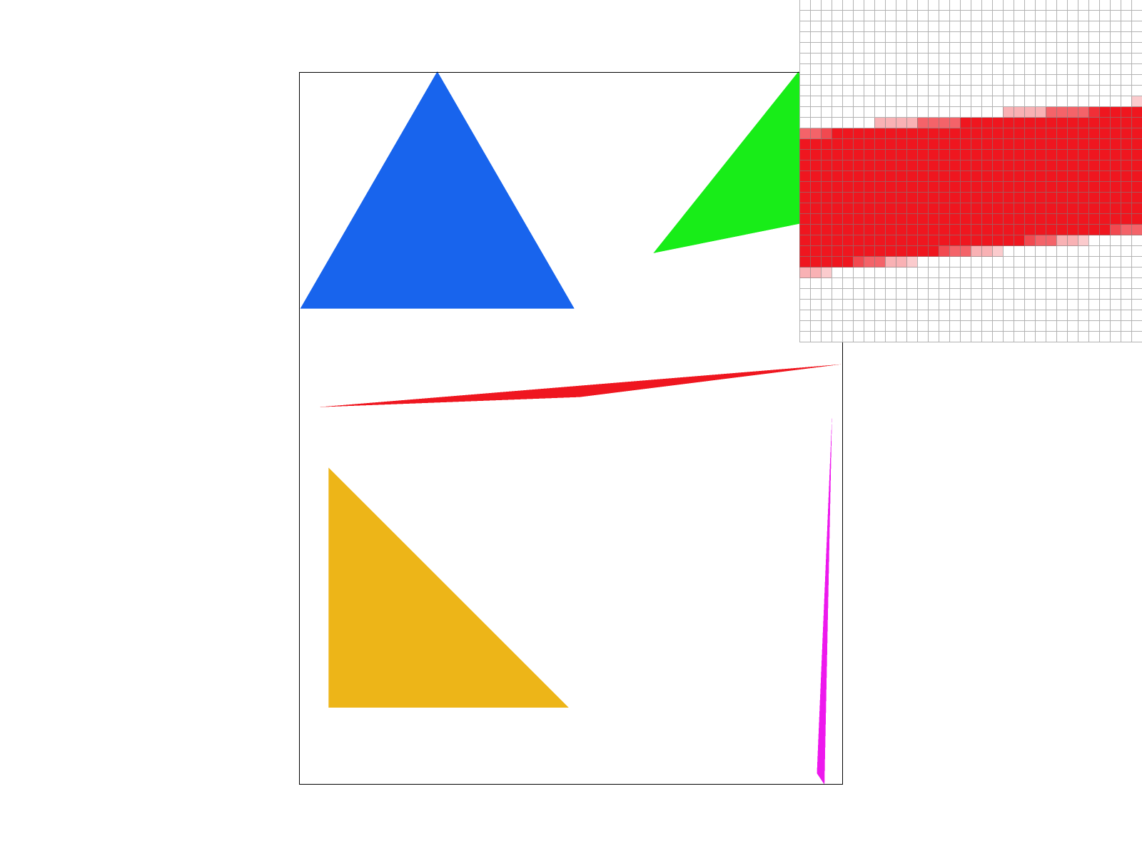
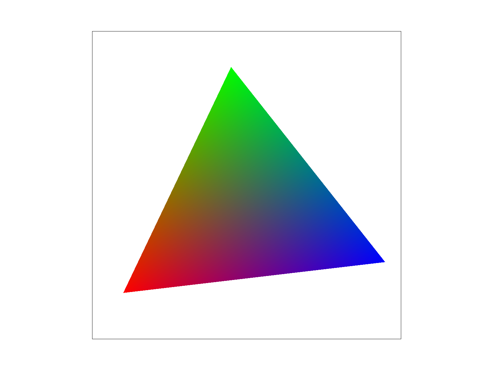
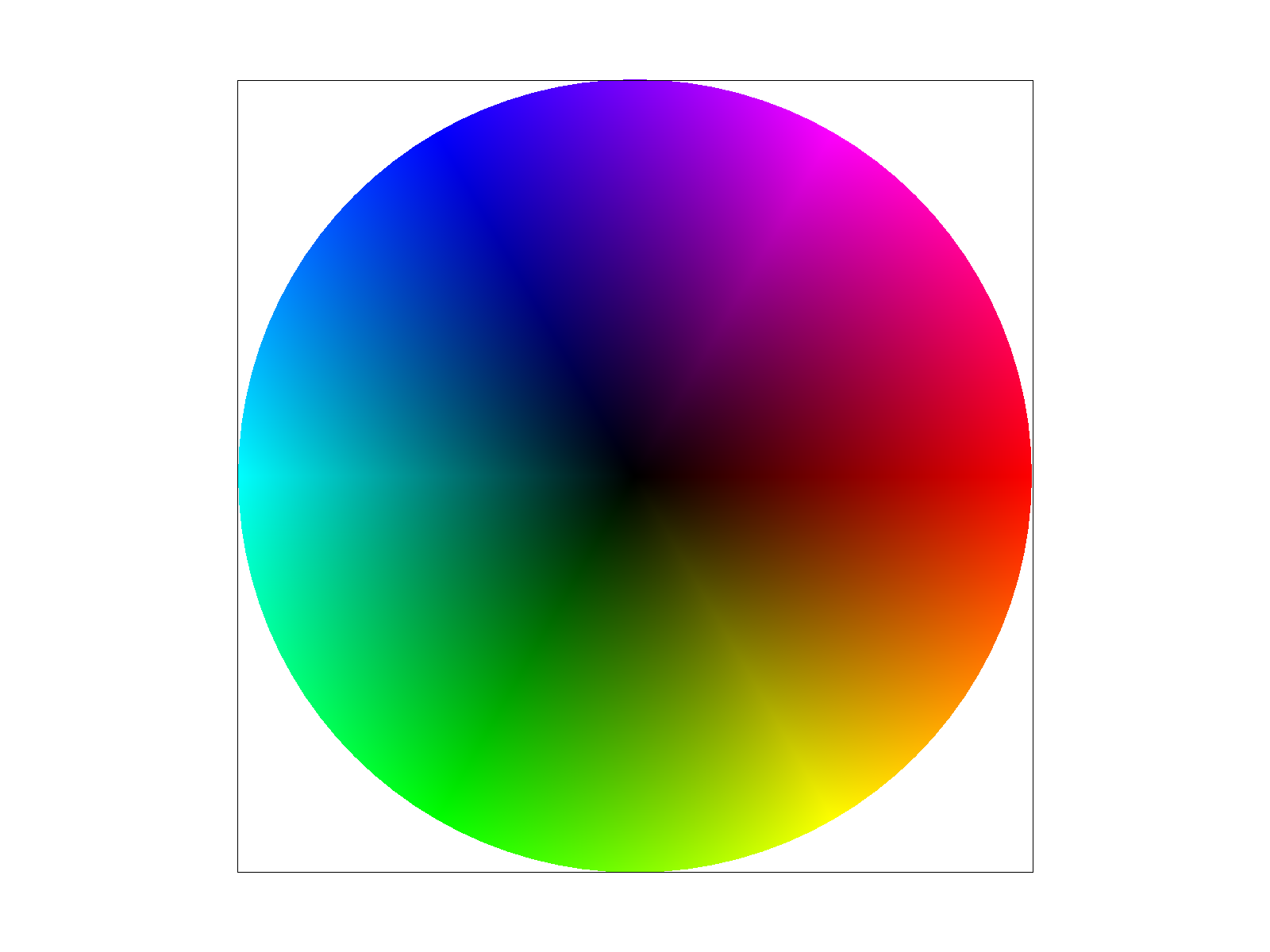
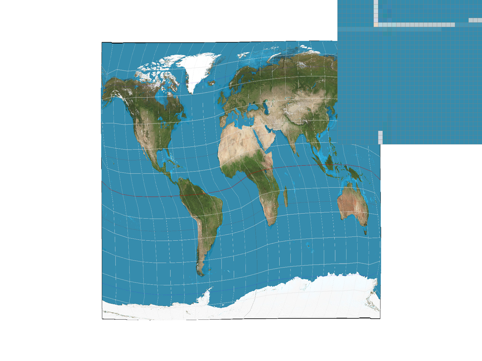
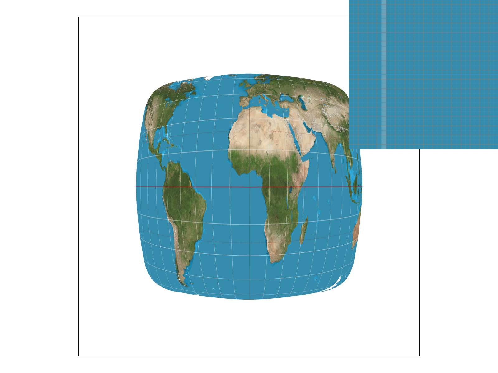
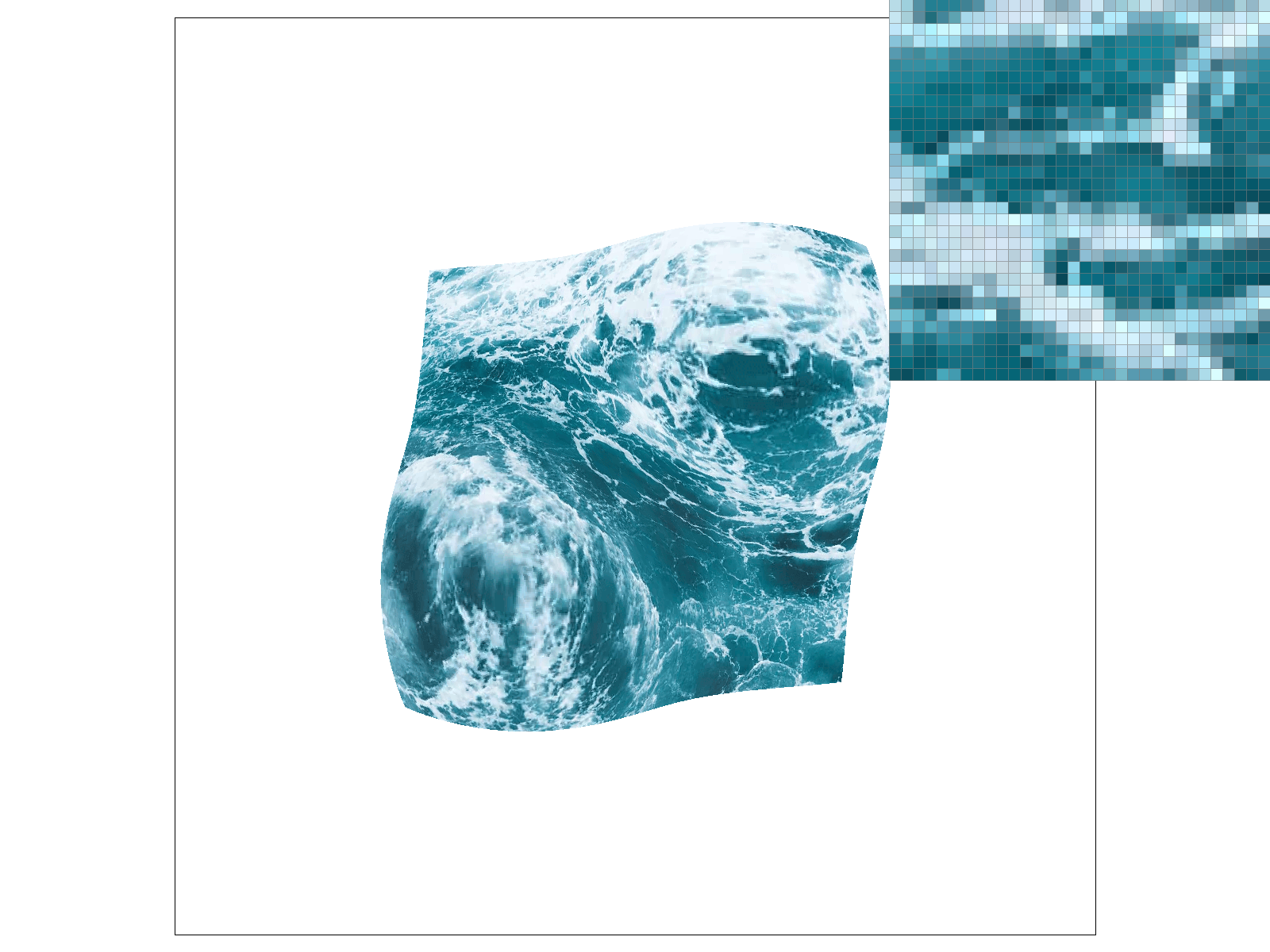
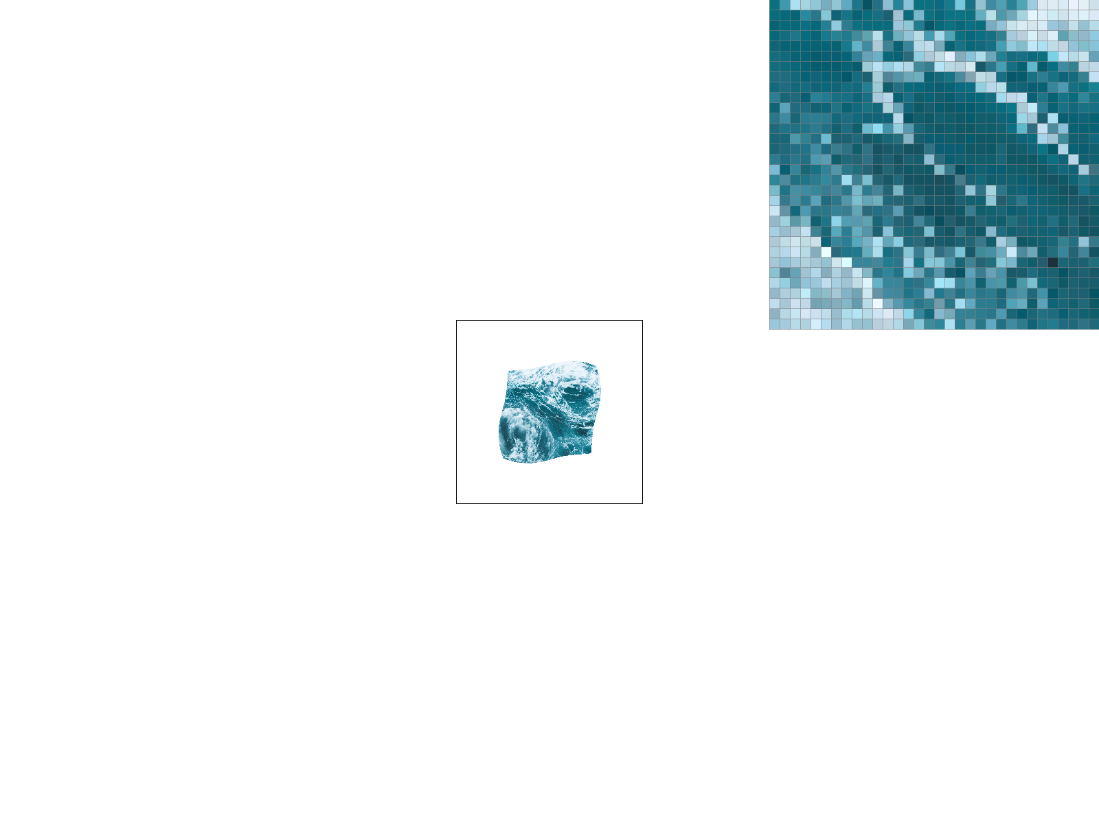
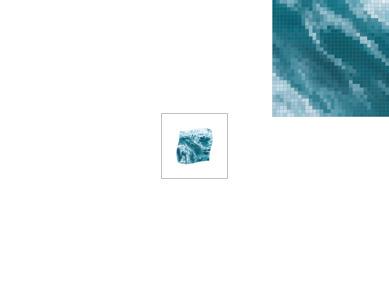
We also calculate the vectors going towards point \(p\). So we just have to check if \(p\) lies on the left of each oriented half-plane given by the requirement that: \begin{equation*} v_{i} \cdot n_{i} \leq 0 \end{equation*} This means that drawing triangles to the frame buffer starts by computing the bounding box, and iterating through the rows and columns to perform this check. Here are some results:

Supersampling

Two of the images in the previous section contain a major flaw related to aliasing. Because we do not sample at a high enough rate, jaggies on the triangles and edges of the cube are visible:

To fix this, we increase the sample rate from 1 sample per pixel. This means expanding the sample buffer, to account for our new samples, running the point in triangle check, and downsampling by averaging the values in each pixel to go from sample buffer to frame buffer:

The resulting edges of the triangles are smoother and jaggies become less of an issue. Hover over the images to zoom in:

Transforms

To draw various triangles at different locations, we can utilize transforms to rotate, scale, and translate a triangle. This is known as an affine transformation and can be broken down by: \begin{equation*} \begin{bmatrix} R & T \\ 0 & 1 \end{bmatrix} \end{equation*} Where the top left matrix is the rotation matrix and to the right is the translation matrix.

Barycentric Coordinates

Through barycentric coordinates, we have a nice way of interpolating across the plane of a triangle. Given the points \(p_1, p_2, p_3\) of a triangle, we can represent any point in the interior of the triangle as a linear combination of these points. With weights \(w_1, w_2, w_3\), we would just require that\begin{equation*} w_1 + w_2 + w_3 = 1\end{equation*}and\begin{equation*}w_1, w_2, w_3 \geq 0\end{equation*}This means that we can use these weights to interpolate color across the plane of a triangle, where if a point \(p = w_1p_1 + w_2p_2 + w_3p_3\) were inside the triangle, its color value would be: \(w_1c_1 + w_2c_2 + w_3c_3\)

Where \(c_1, c_2, c_3\) are the colors corresponding to vertices \(p_1, p_2, p_3\)

Sampling Pixels for Texture Mapping

To map textures onto triangles, we can use the \(uv\)-coordinate system. Both \(u, v\) represent the coordinates of points on the texture, which scale from 0 to 1, and represents the normalized scaling of the texture. Since the vertices of the triangle are each assigned a \(uv\) coordinate, we can perform barycentric interpolation to find the \(uv\) coordinate of every vertex inside the triangle. And to find the color of the pixel, we would just perform sampling on the texture given the uv coordinates.

Nearest Neighbor Filtering

In nearest neighbor filtering, given the four closest pixels to the \(uv\)-coordinate (scaled up to height/width of texture), we would choose the closest pixel and return the color of that pixel for our texture mapping.

Bilinear Filtering

In bilinear filtering, we consider the 4 closest pixels to our sample point. Then along both axis, we perform a linear interpolation between the colors in each axis.

Level Sampling with Mipmaps

Overview

Another anti-aliasing technique we can add on top of the previous ones is level sampling, in which for objects far away, we can sample from a lower resolution texture. This relieves the problem of failing the sample high frequencies for objects far away in which there are not enough pixels to sample into.

To do this, we compute the partials of the \(uv\)-coordinates with respect to \(xy\)-coordinates, and base the resolution of the texture we want to sample from off of that. This just means that if the triangle we are rasterizing is large with respect to our texture, we want to sample from a full resolution texture, while if the triangle is small wrt to the texture, we want to sample from a downsampled texture.

Implementation

As for the implementation details, we compute the barycentric coordinates for \((x, y), (x + 1, y), (x, y + 1)\) in our triangle to rasterize and apply the interpolation to get the cooresponding \(uv\)-coordinates, \((u, v), (u_x, v_x), (u_y, v_y)\). We see that \((x + 1, y) - (x, y)\) gives a 1 unit change in the \(x\) direction, so \((u_x, v_x) - (u, v)\) gives the change in \(u, v\) with respect to \(x\). We do the same with respect to \(y\), and compute \begin{equation*}L = \max\left(\sqrt{\left(\dfrac{du}{dx}\right)^{2} + \left(\dfrac{dv}{dx}\right)^{2}}, \sqrt{\left(\dfrac{du}{dy}\right)^{2} + \left(\dfrac{dv}{dy}\right)^{2}}\right) \end{equation*}Then to get the level of the mip map, we take the log of this value:\begin{equation*} d = \log_{2}{L} \end{equation*}

It is difficult to see the difference across the level sampling methods, but the effect is more noticeable when we zoom out, as aliasing becomes a problem. Hover over the following three images to zoom in: