In this project, we explore ways of working with bezier lines/curves along with understanding the data structures needed to perform mesh operations. It was great to learn about the data structures we can use to traverse the mesh and modify parts of it locally.
Bezier Curves
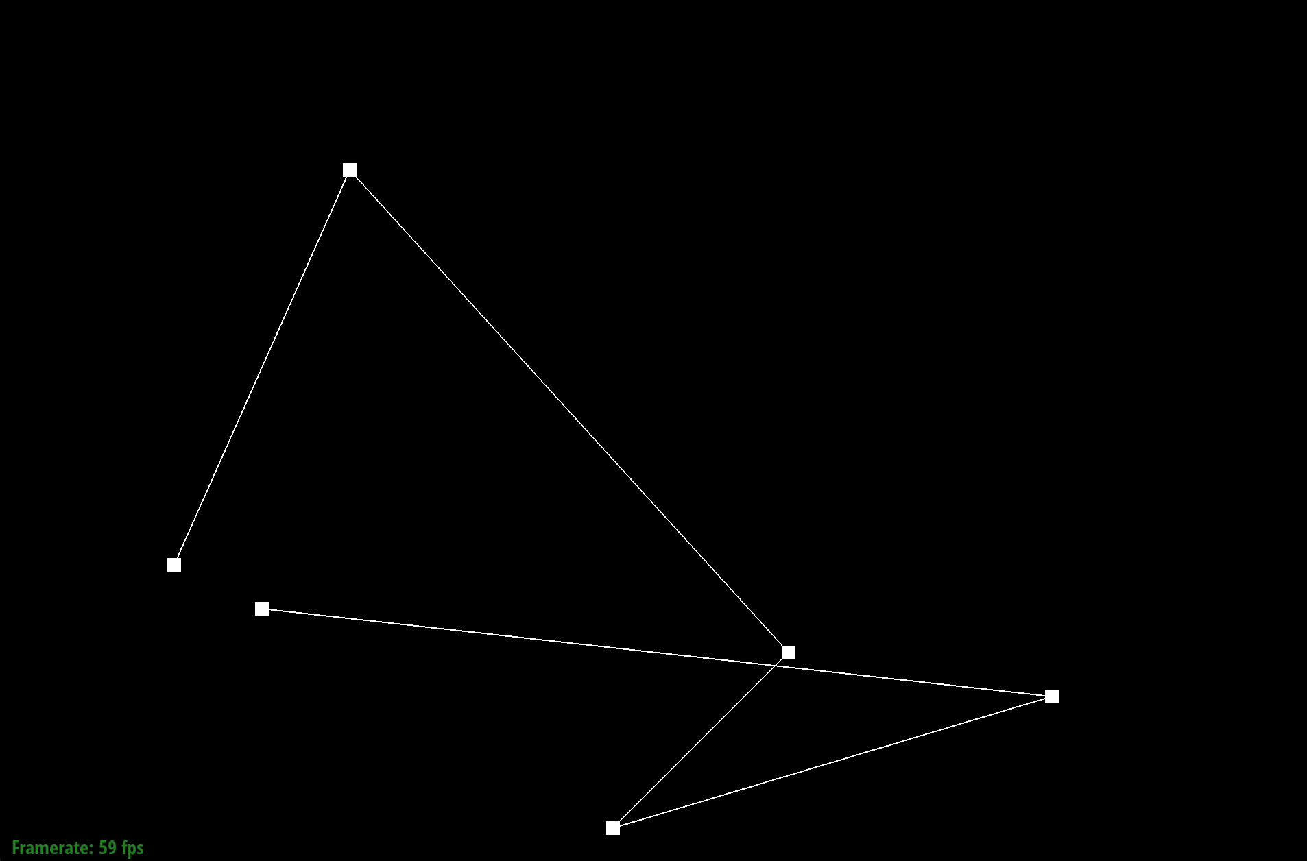
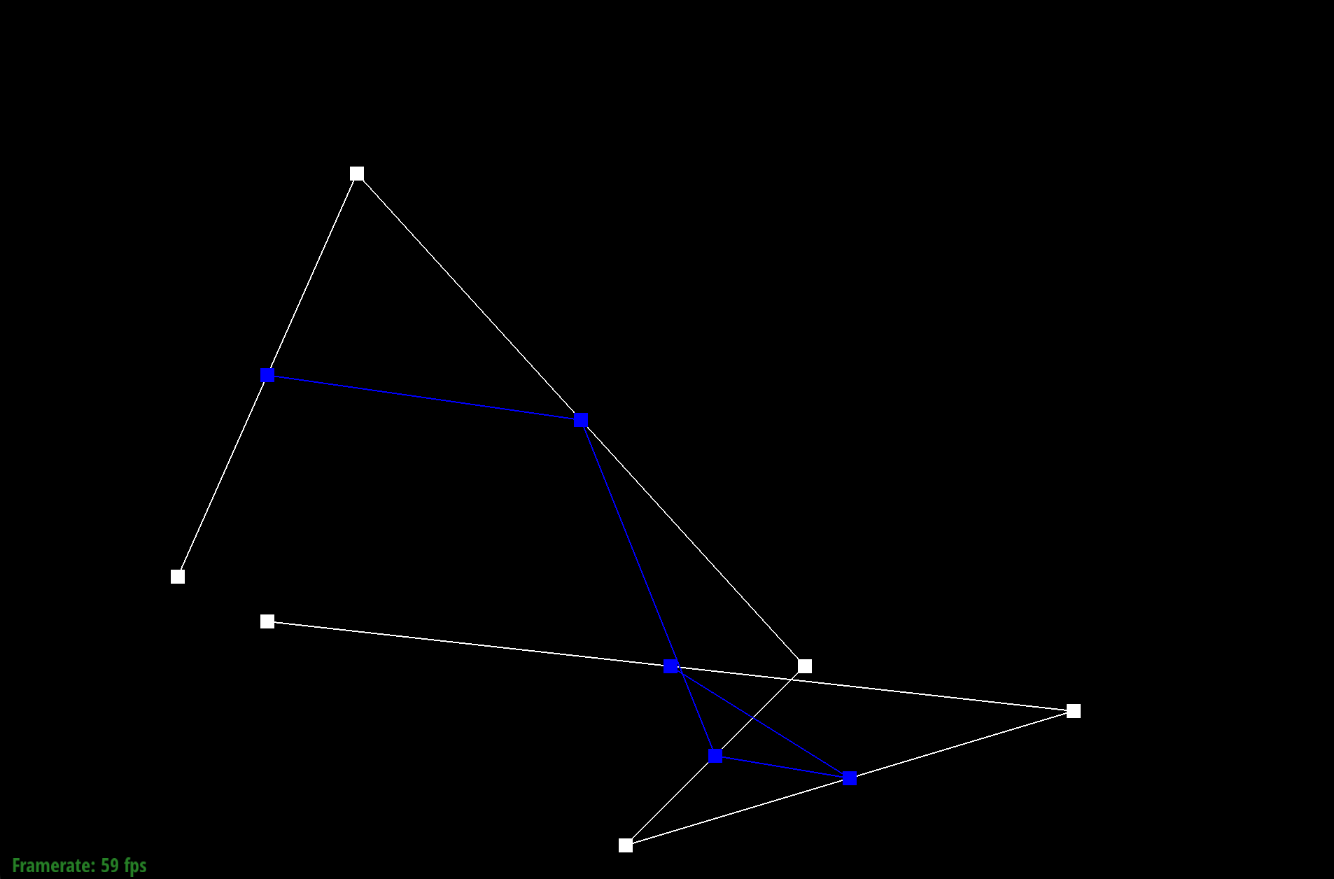
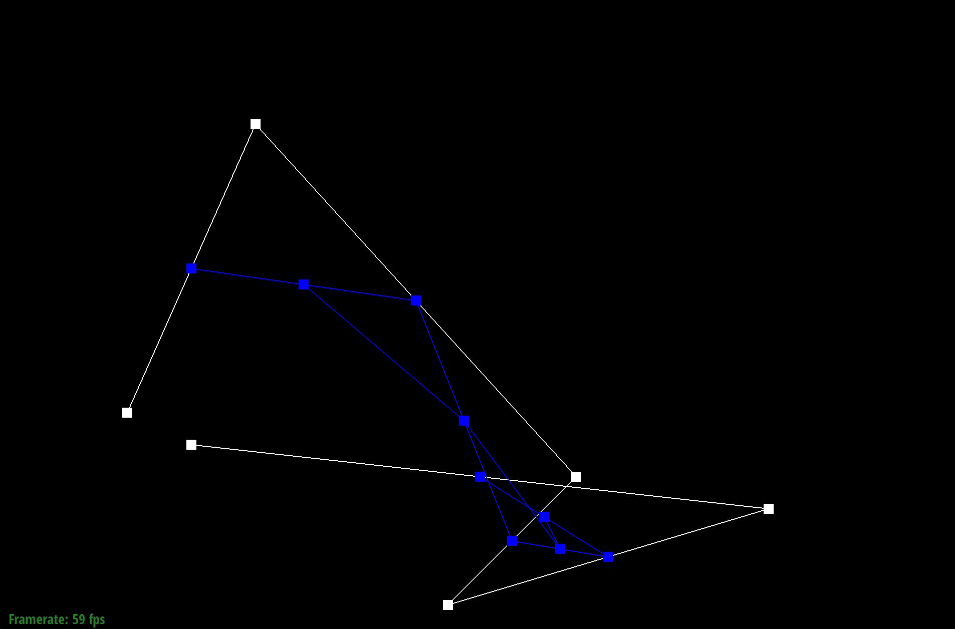
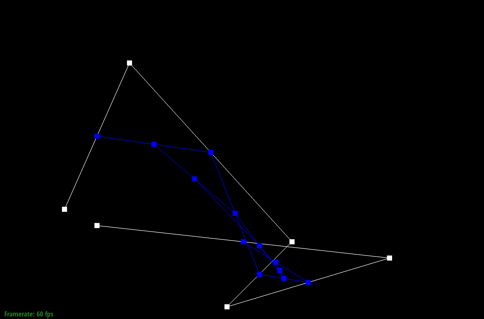
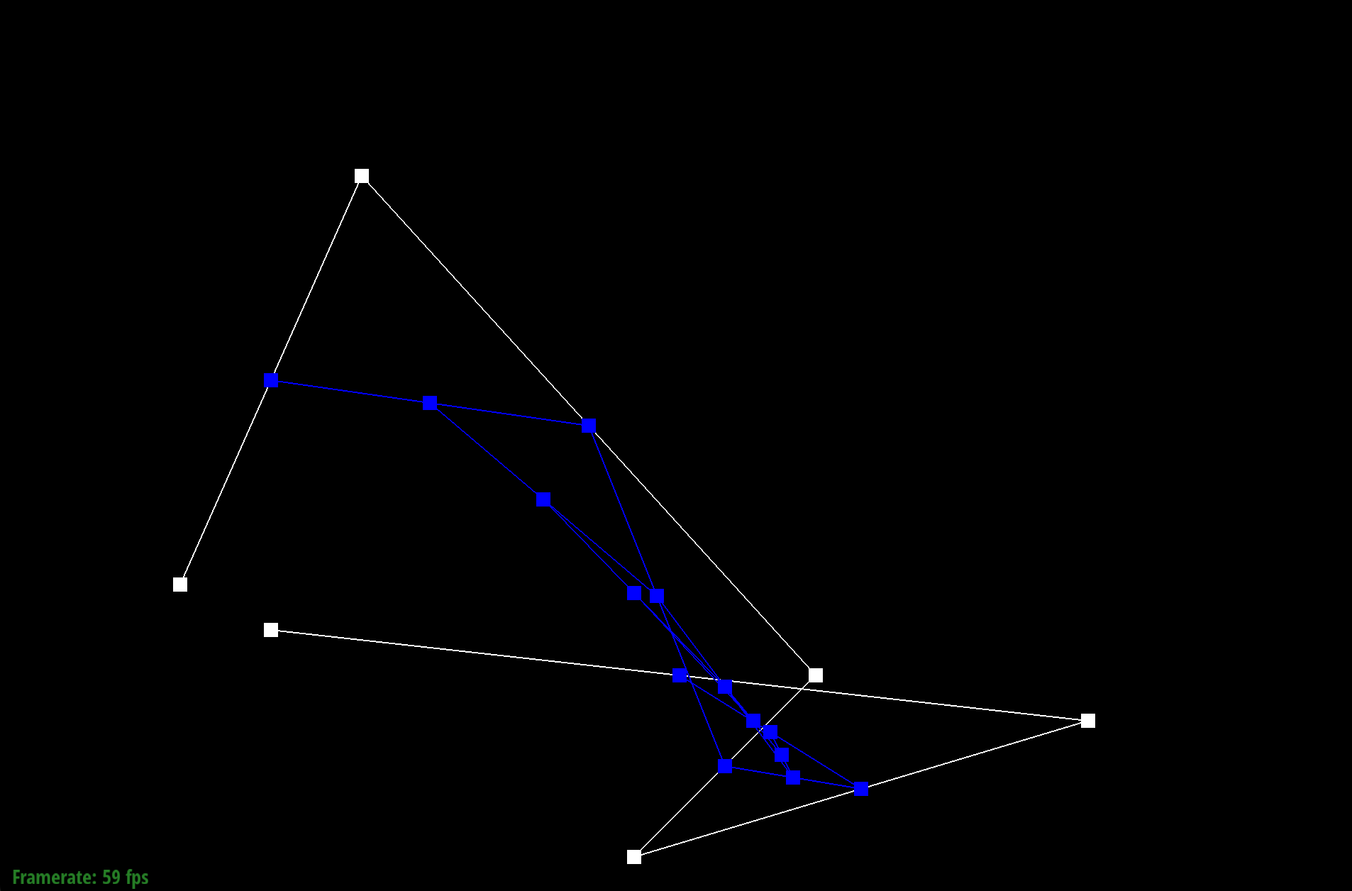
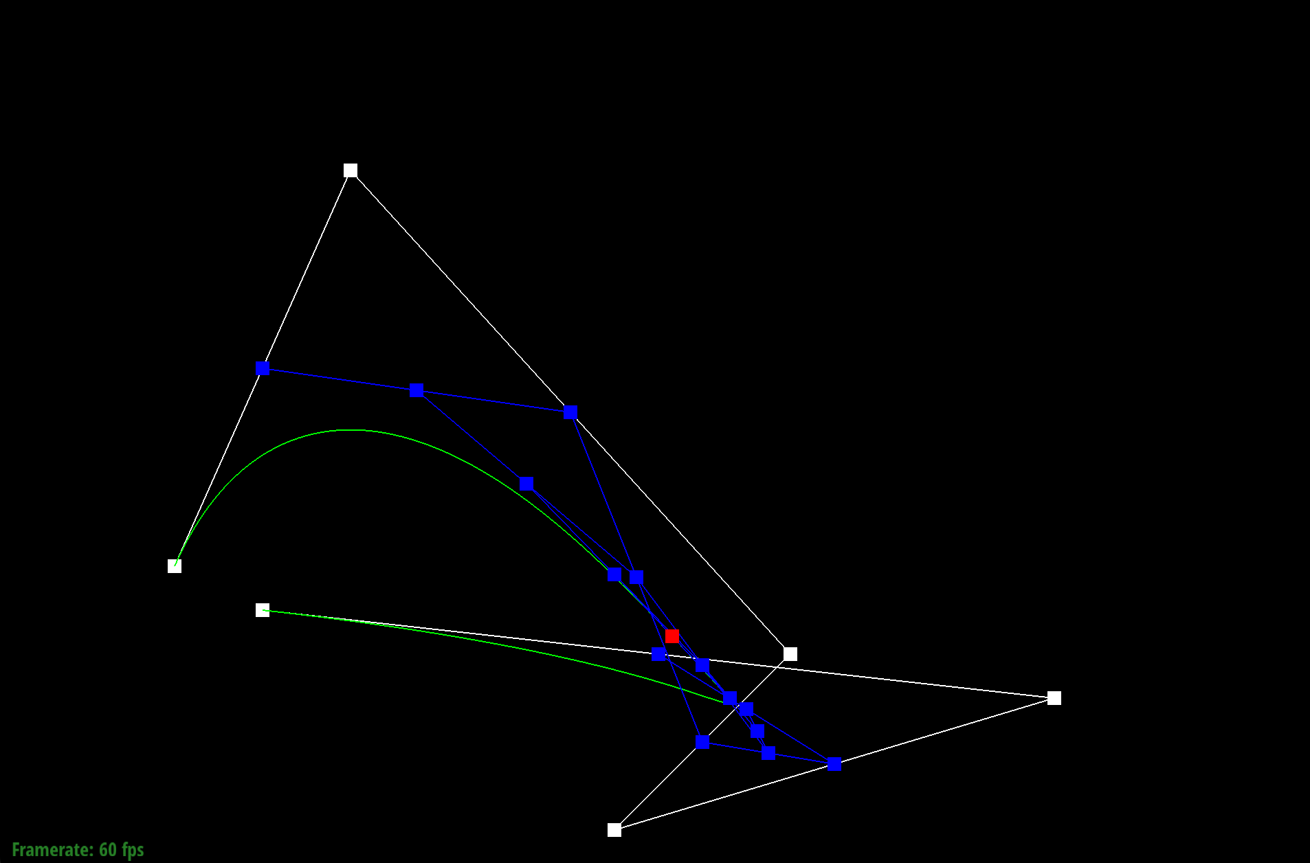
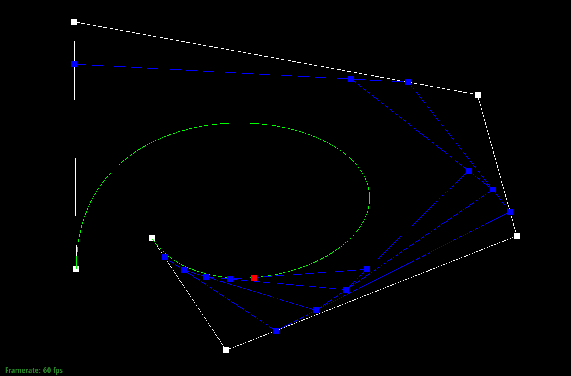
In Casteljau's algorithm, we compute a series of lerps until the number of control points goes down to 1. This last point will be a point on the curve. This gives a recursive/iterative algorithm for computing the point. We are given a vector of points and compute a lerp on that vector to get a new vector of control points, repeating until our final vector has 1 point. The \(t\) parameter we use for interpolation remains constant for a given point we want to compute on the curve. The images below illustrate the steps for computing the Bezier curve given 6 control points. Hover over the images to zoom in:
Step 1 Step 2 Step 3 Step 4 Step 5 Step 6
And here is an example where we moved a control point and set \(t\) to a new value.
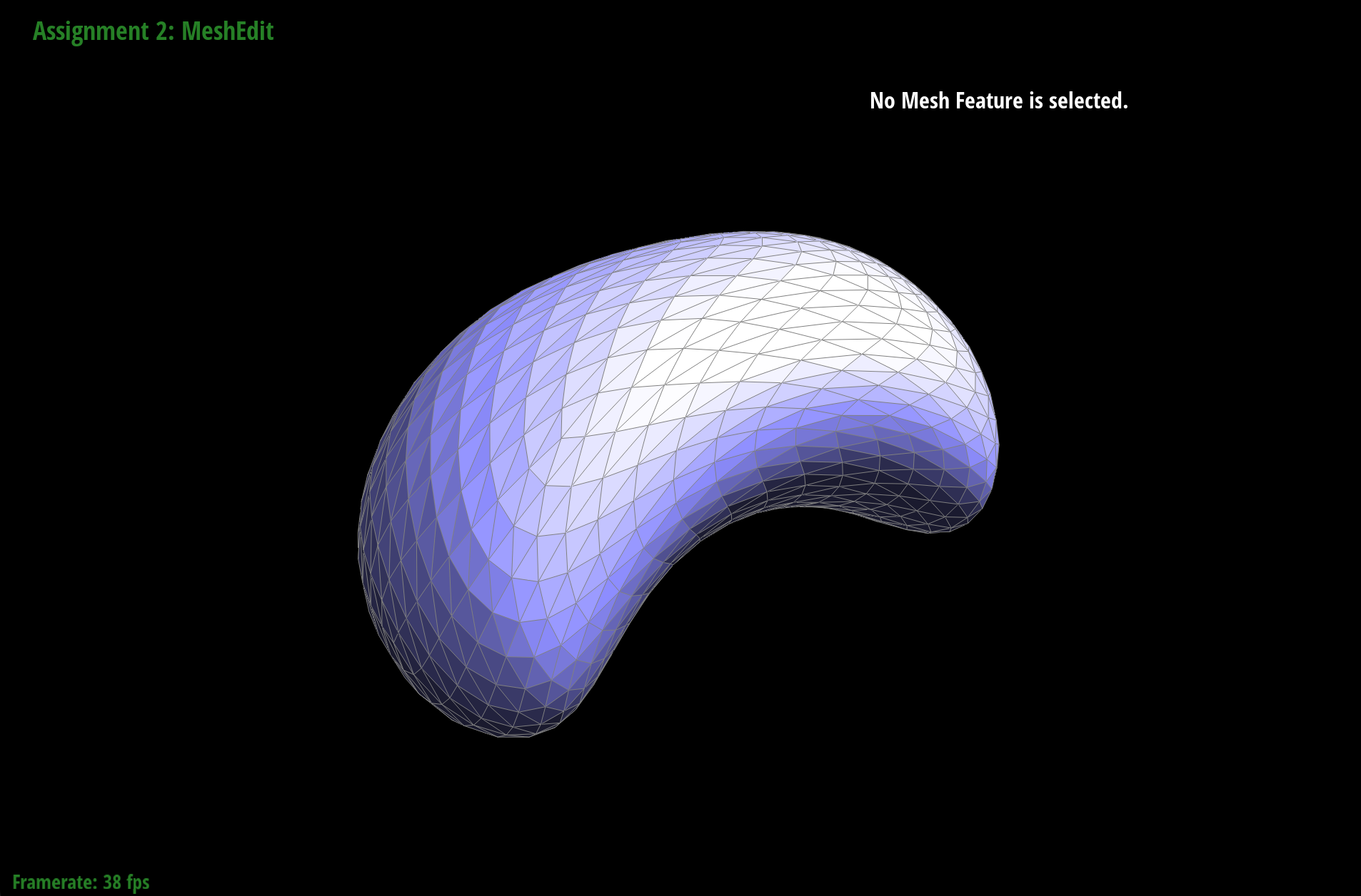
Bezier Surfaces
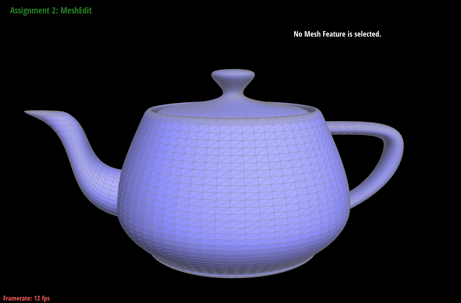
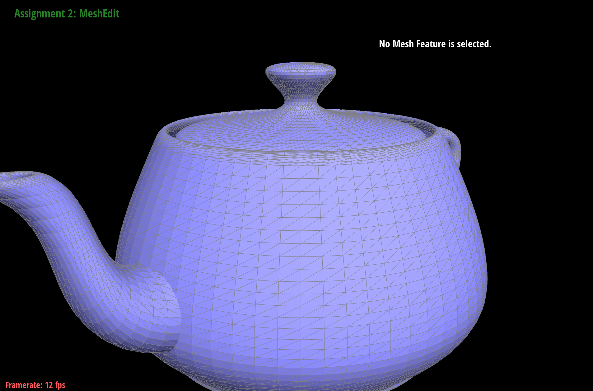
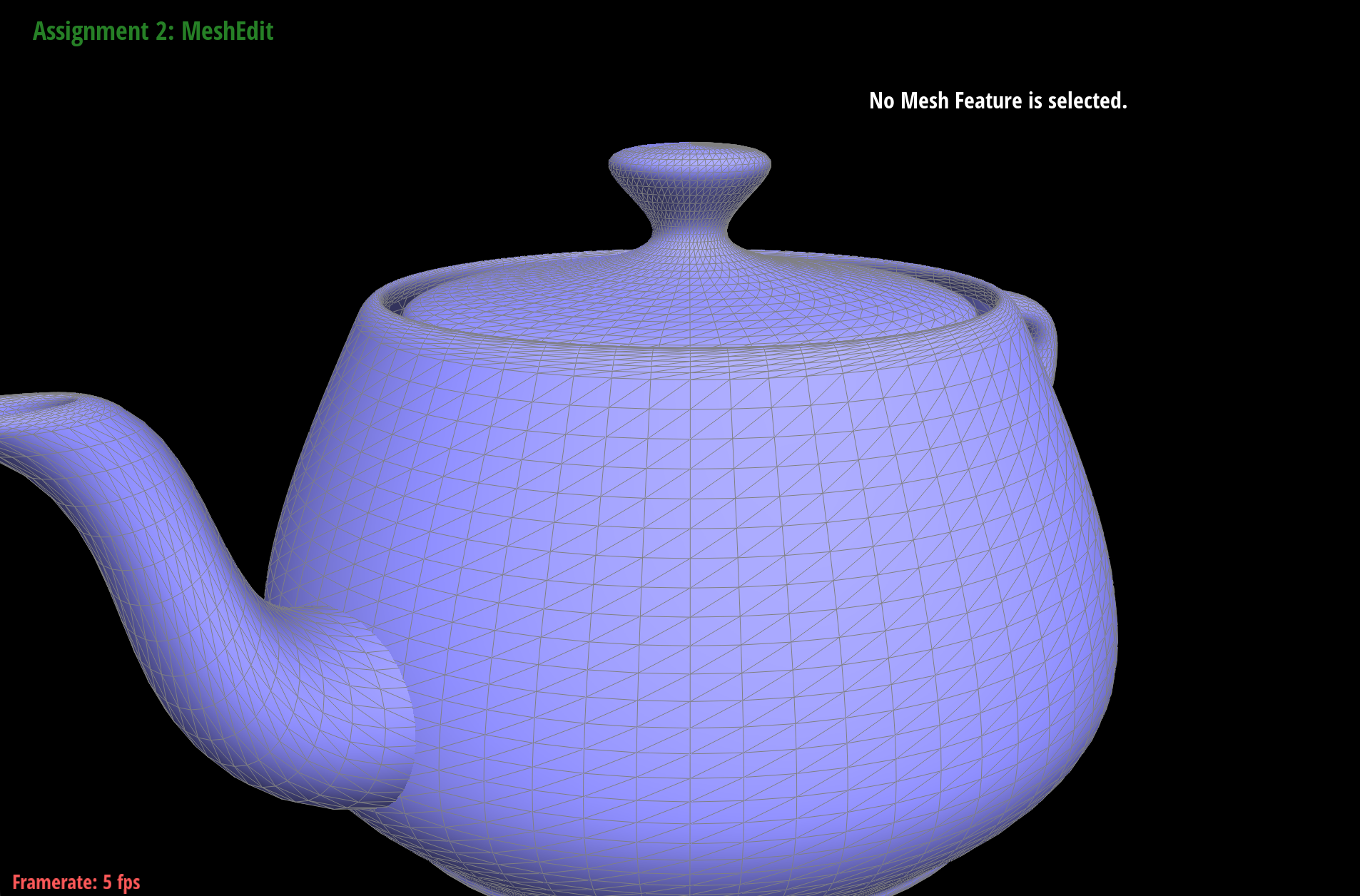
For bezier surfaces, we are now given a 2-d array of control points and two parametric variables, \(u, v\) where \(u\) represents the fraction along the \(x\)-axis and \(v\), the \(y\)-axis. To find a point on the curve given \(u, v\), we first collapse along one dimension by fully running Casteljau's algorithm for control points share the same \(x\)-coordinate, using \(u\). Then we collaps along the second dimension, for ones sharing the same \(y\)-coordinate, this time using \(v\). Teapot:
Area Weighted Normals
To calculate the normals at the vertices of the mesh, we take a weighted sum of the normals associated with the faces around that vertex. To traverse the faces, we iterate around the half edges of the center vertex. Then we get the face associated with the halfedge:
To weigh the normals, we can take 1/2 of the norm of the cross product between two vectors of the face:\begin{equation*} \dfrac{1}{2} \lVert v_{1} \times v_{2} \rVert \end{equation*}and multiply scale the normal by this area. Finally, we take a linear combination:\begin{equation*} v_{\perp} = \sum {Area}_{i} * n_{i} \end{equation*}and normalize. Using the normals, we can have better shading by interpolating the shading value across each triangle surface (hover to zoom in):
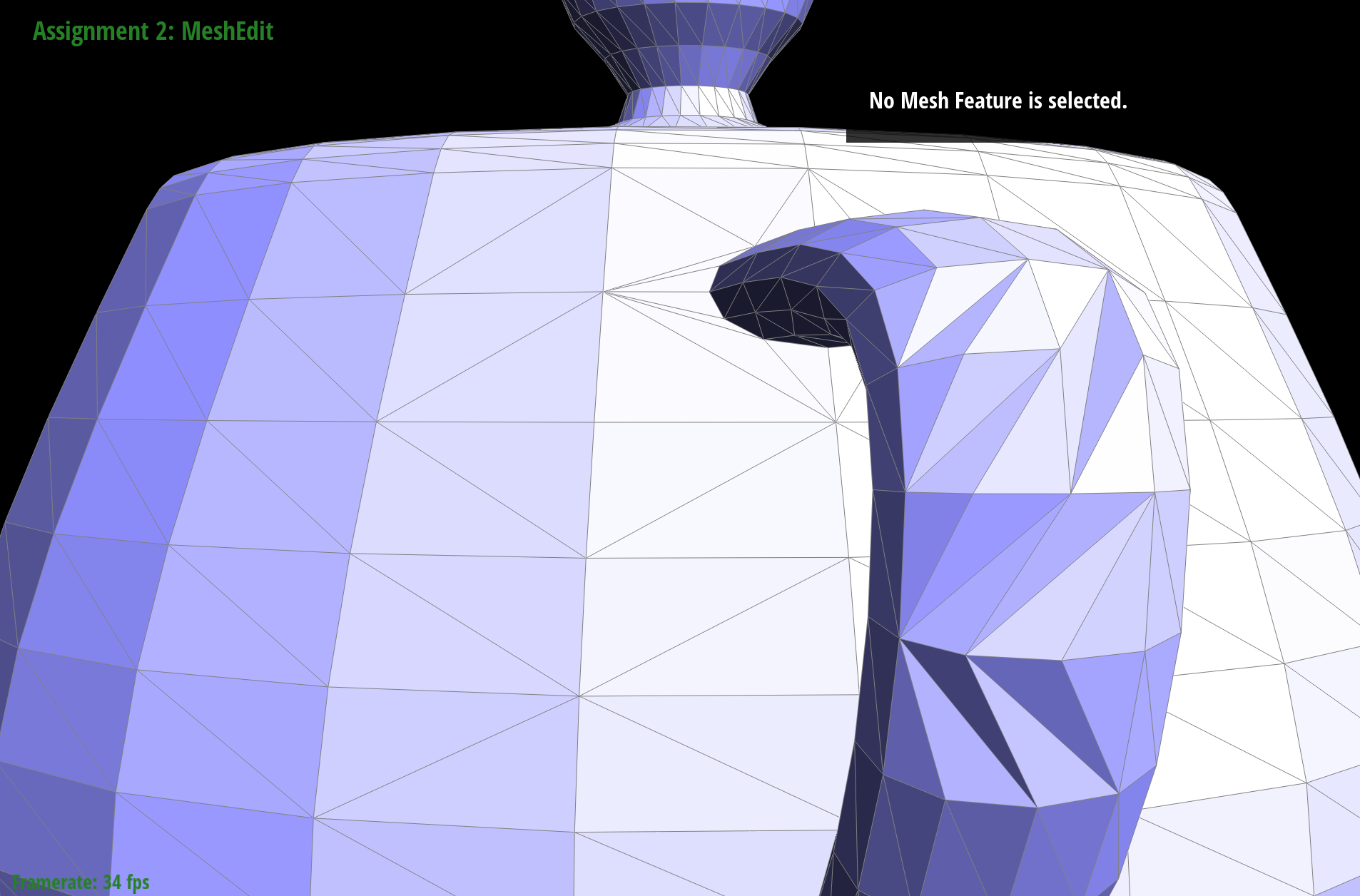
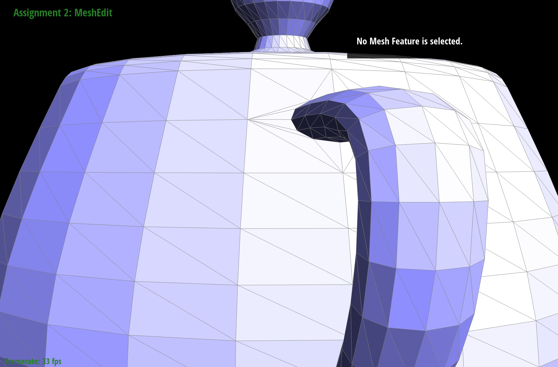
Flat ShadingPhong Shading
A difference we see is that with the flat shading, the brightness across each triangle edge has a harsh transition, while for phong shading, it is much smoother.
Flipping Edges
Flipping edges is a local remeshing operation which does not require adding/deleting elements, shown below:
To implement this, we would do pointer reassignments to all elements involved in the component. Here is a list of all variables we need to change in each class:
For halfedges, we can use the setNeighbors method to quickly update all its variables. Here is an application of the function on a couple of edges. Also, hover over the image to see the original edges:
For debugging, it was very helpful drawing out the operations and keeping track of all the variables I needed to update. Keeping the operations symmetrical between the halfedges that I flipped also proved to be convenient.
Splitting Edges
Splitting edges requires more pointer reassignments, and we would have to add more items to our mesh. Here is what the operation looks like:
We would have to create a new vertex bisecting the edge, three new edges to have 4 center edges, 6 new half edges for each of the 3 edges, and 2 new faces. Here is an application of some splits and flips. Hover over the images to view the original mesh before the operations.
Cow Edge SplitsRing Edge Splits and Flips
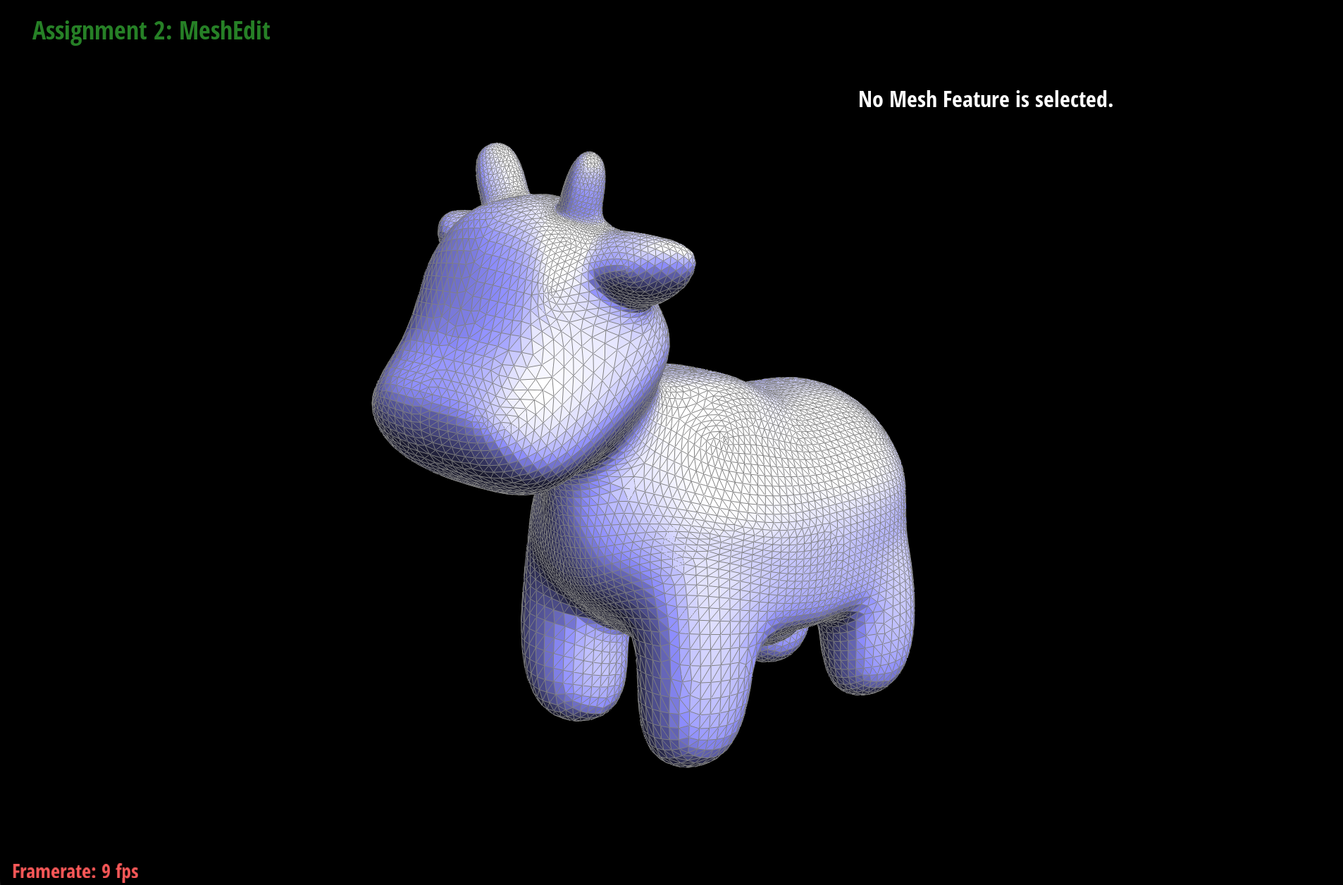
Loop Subdivision
Loop subdivision requires a combination of the previous two operations, the edge split and the edge flip. The process involves splitting all non boundary edges first, the flipping the added edges that connect an old vertex to a new vertex.
Following the diagram, the old edges are marked with green, with the new vertex from the split marked as red. We see that all edges that are green are split by the midpoint, and in the flip run, we fip all black edges that connect a black vertex to a red vertex (non-boundary). Now we can apply this subdivision method to some meshes:
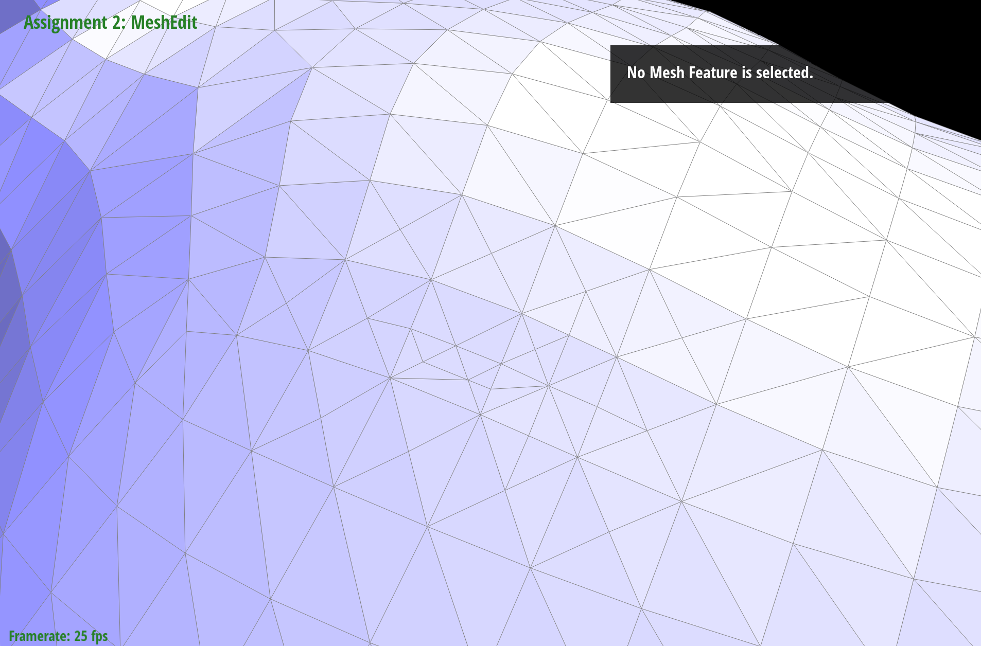
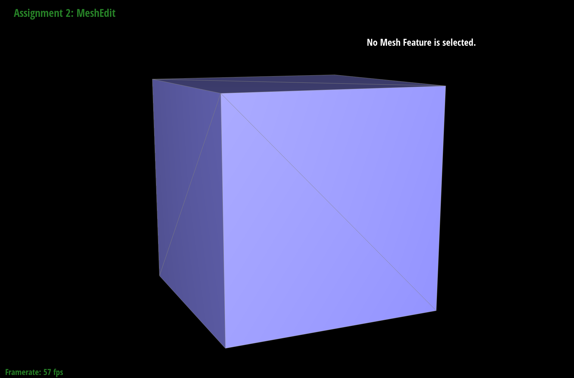
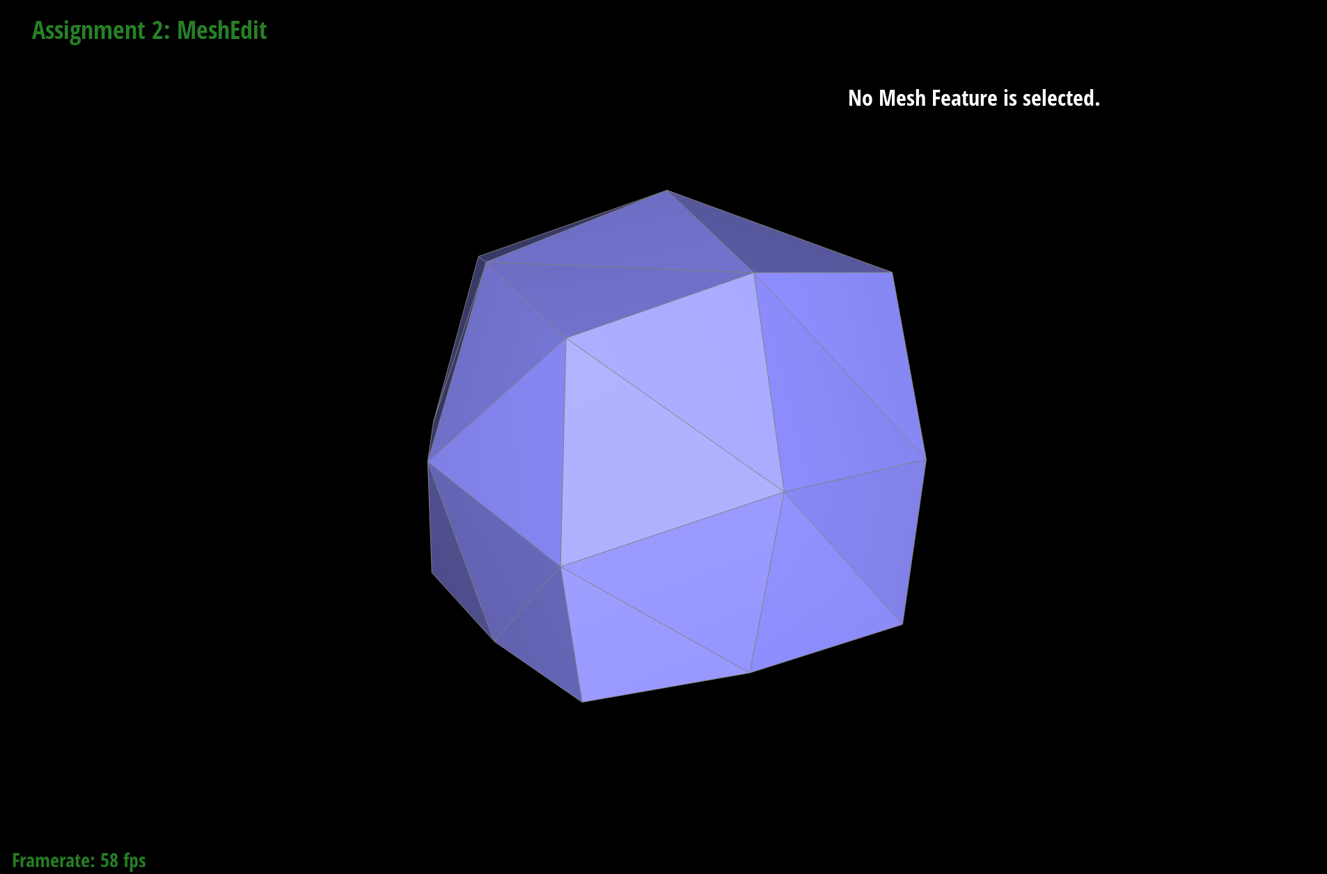
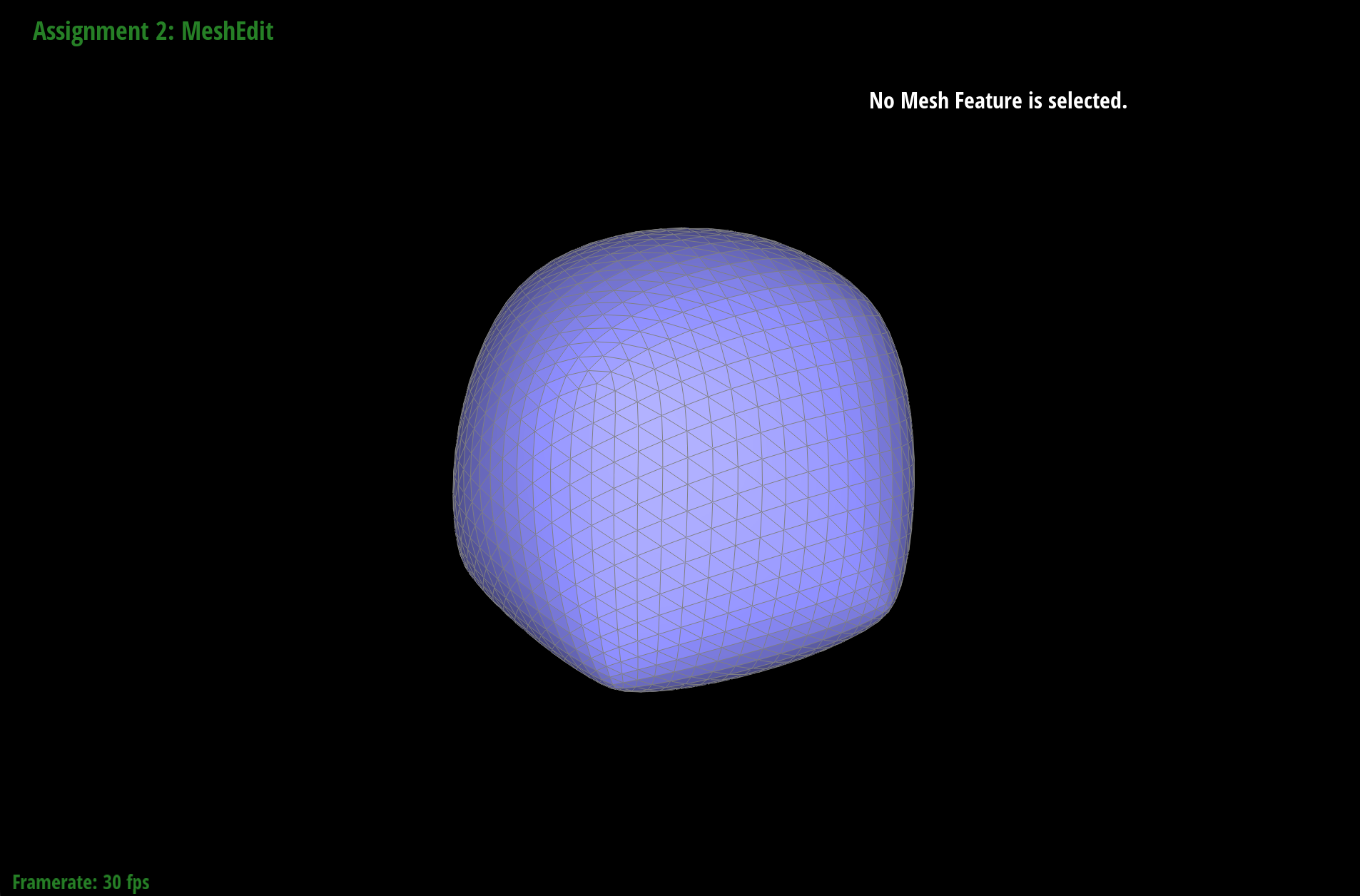
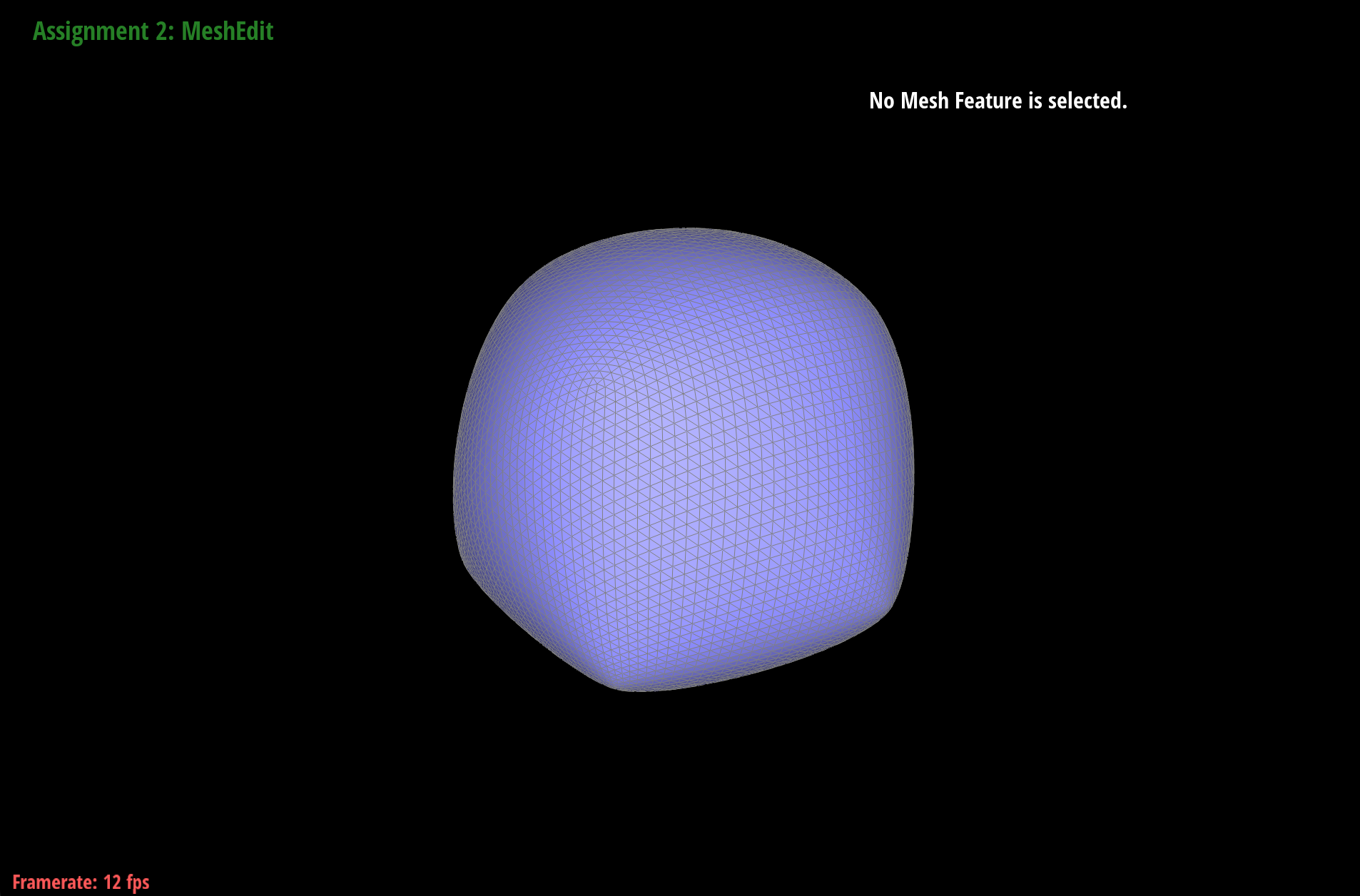
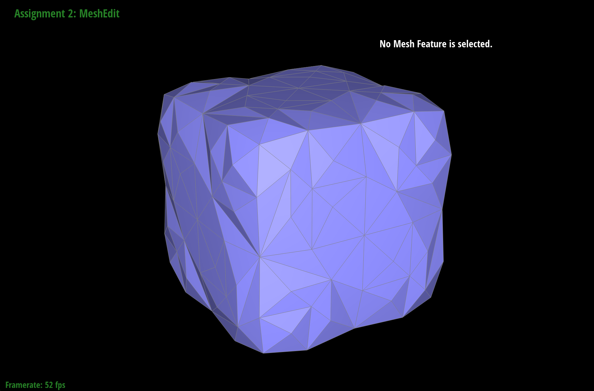
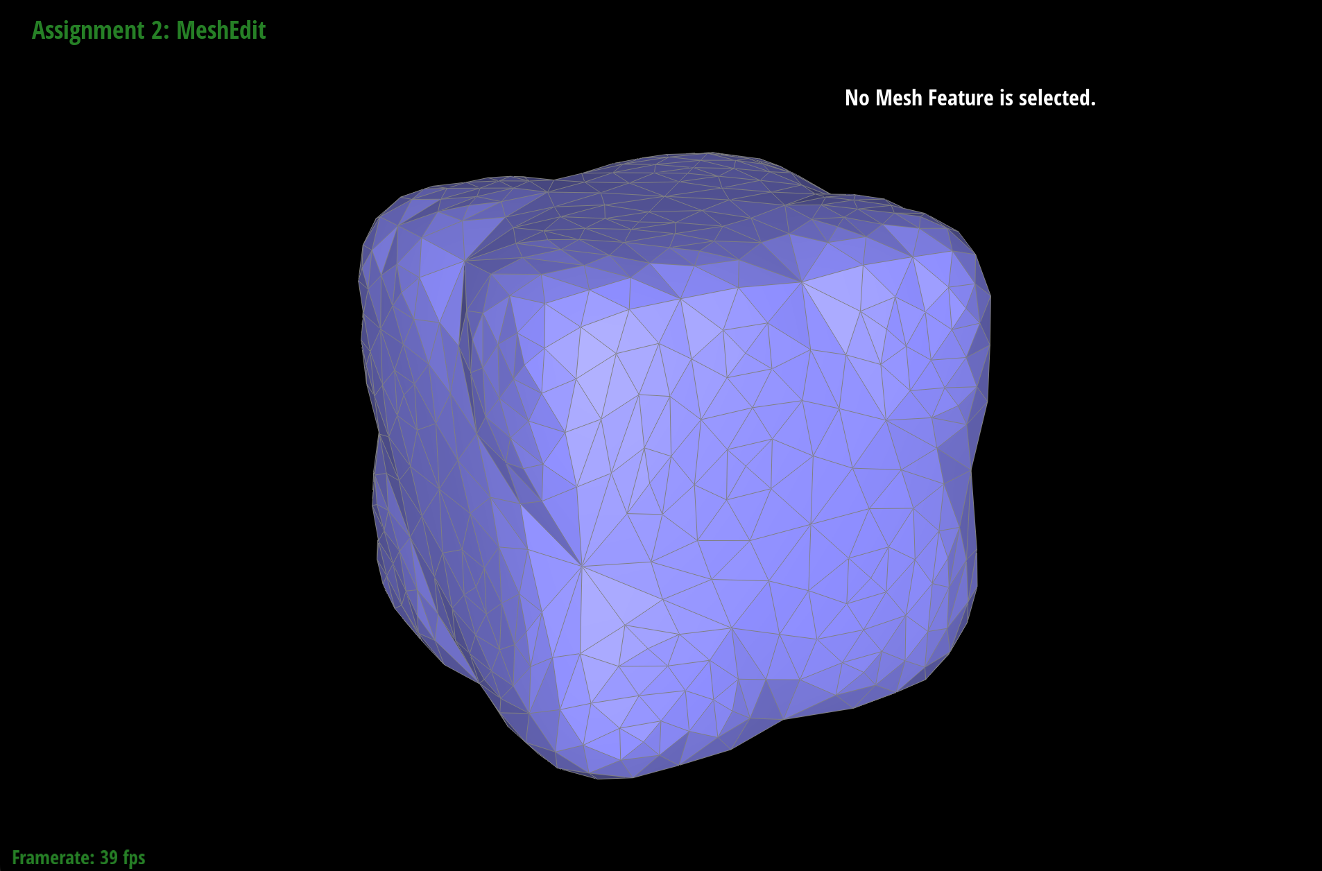
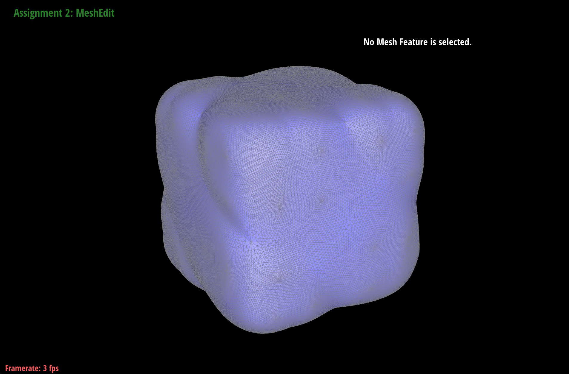
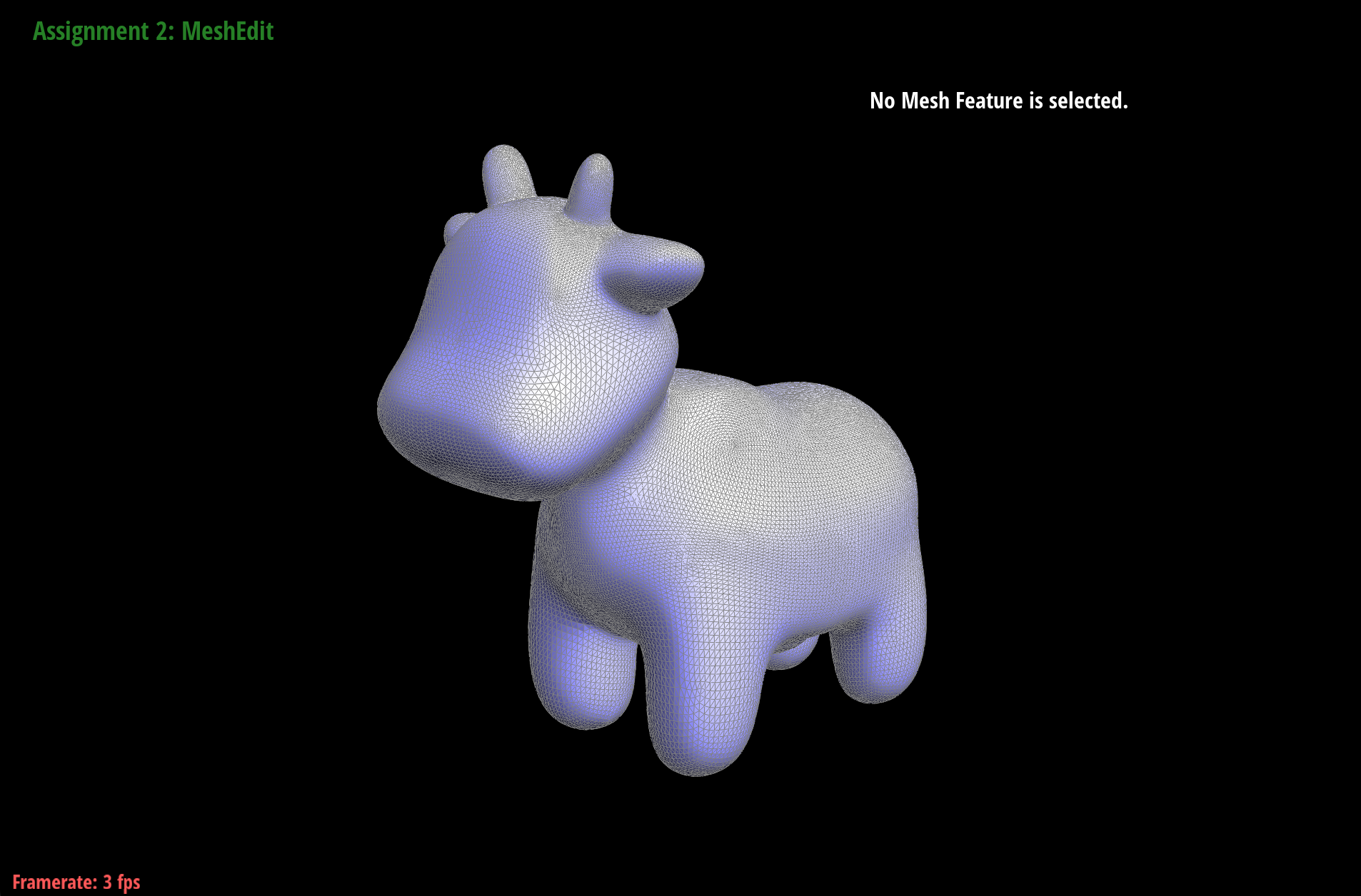
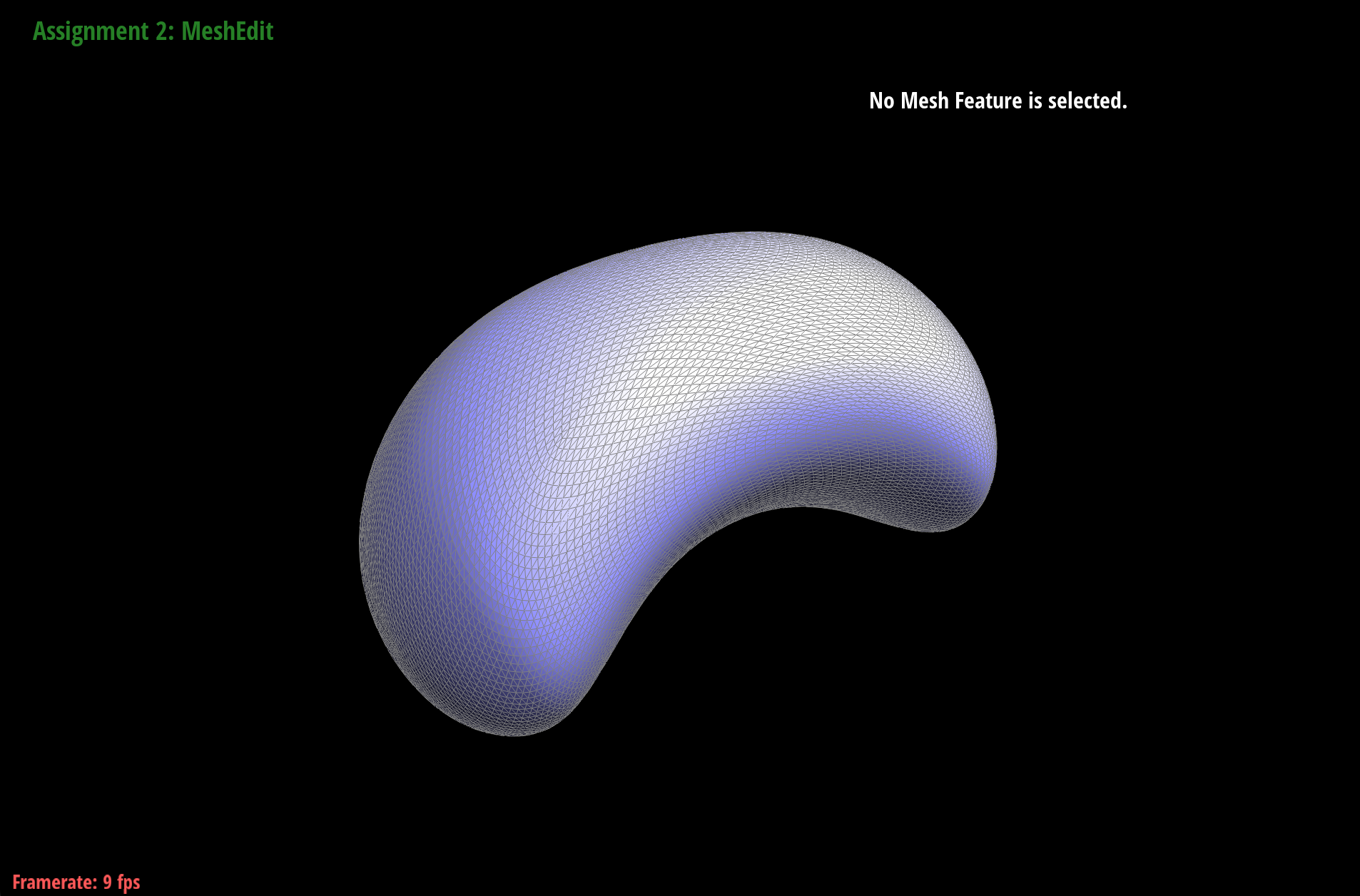
We notice that in subdivision, corners and edges are smoothed out, where the cube's features are rounded. Something we can do to reduce this effect is subdividing the edges such that the cube is made of more triangles. Because loop subdivision calculates the new position of each vertex by its neighbors, we want the neighboring vertices to be close:
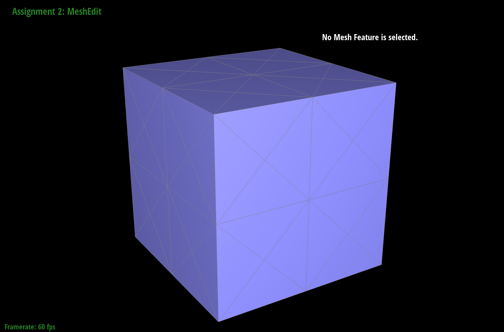
And the result looks more like a cube. The way I also subdivided the edges of the cube gives symmetrical resulting mesh, because along the face of the cube, the diagonal splitting each face into triangles can go from top right to bottom left, or top left to bottom right. By adding diagonals such that the mesh is symmetrical, we get a symmetrical subdivision.
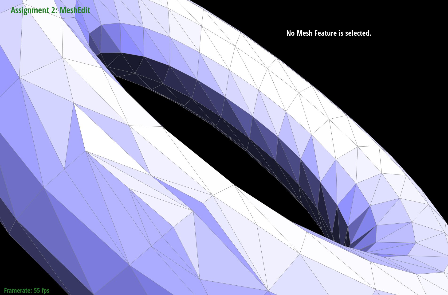
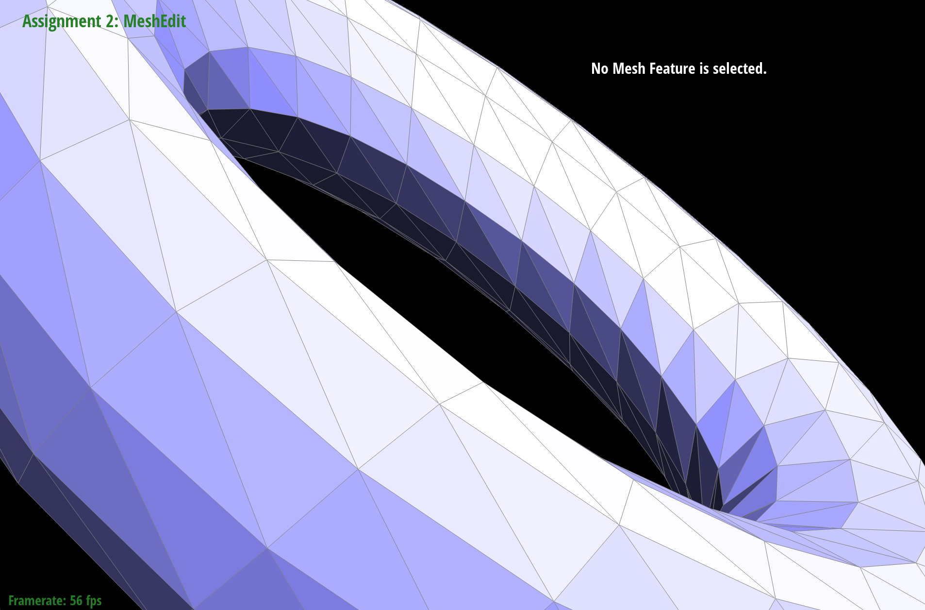
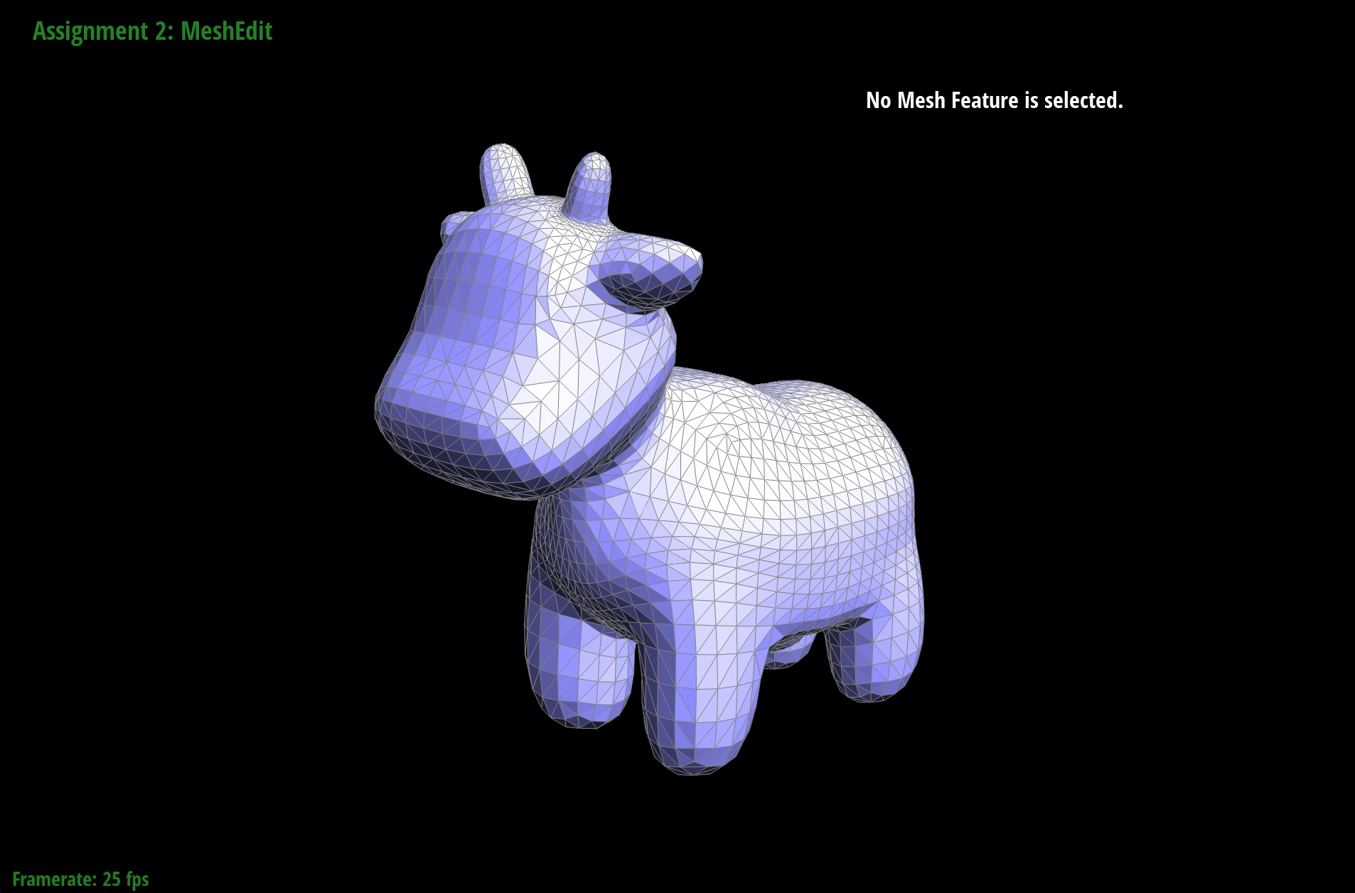
Lastly, here is the algorithm applied to more interesting meshes: