In this project, I have implemented methods simulate light in a scene and have explored ways to speed this up using a bounding volume hierarchy. From completing this assignment, I got a better grasp of how light interacts with objects and how different materials are rendered.
Ray Generation and Scene Intersection
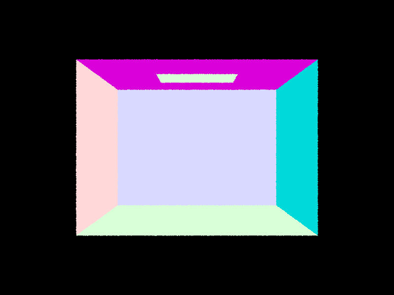
To generate the camera rays for our scene, we normalize our image coordinates which we use to calculate the rays from the camera based on the vertical and horizontal field of views. The bottom left corner of the camera sensor is given by\begin{equation*} bl = \left(-\tan\frac{hFov}{2}, -\tan\frac{vFov}{2} \right) \end{equation*}and for the top right, we get:\begin{equation*} tr = \left(\tan\frac{hFov}{2}, \tan\frac{vFov}{2} \right) \end{equation*}So if we have a point \(x, y\) on the image, it would be a linear interpolation between the bottom left point and top right:\begin{equation*}bl + (x(tr - bl)[0], y(tr - bl)[1]) \end{equation*}
Next would be intersection the ray with various objects in the scene. The first intersection test would be with a triangle, and the method I used included solving a system of equations for the barycentric coordinates of a potential intersection point. This is known as the Moller-Trumbore algorithm, and we can recover the coefficients by solving the system:\begin{equation*}\begin{bmatrix}\mid & \mid & \mid \\-D & (p_{2}-p_{1}) & (p_{3}-p_{1}) \\ \mid & \mid & \mid \end{bmatrix}\begin{bmatrix} t \\ u \\ v \end{bmatrix} = r.o - p_{1} \end{equation*}From this system, we get \(t, u, v\), and for the last barycentric value, we can take \(1 - u - v\). To check that the ray intersects the object, we require that \(t >= 0\) and that there were no objects closer to the ray that the ray has already intersected with. So we also need \(t <= r.max_t\).
We can also calculate the intersection of rays with sphere since we have the formula for both. The formula for a sphere is:\begin{equation*}\lVert v - s.c \rVert = s.r\end{equation*}And for a ray:\begin{equation*} v = r.o + r.d \cdot t \end{equation*}Then substituting in \(v\) into the sphere equation, we get a quadratic equation and can solve for \(t\) with the quadratic formula:\begin{align*} a &= dot(r.d, r.d) \\ b &= 2 * dot(s.c - r.o, r.d) \\ c &= dot(s.c - r.o, s.c - r.o) - s.r^{2} \end{align*} We check for a nonnegative determinant to get solutions and here is the result of the ray intersection with a sphere:
Bounding Volume Hierarchy
In a bvh, we store objects and their bounding boxes. When we construct our tree out of these bounding boxes, we split the bounding boxes into a left and right set and call our constructor on the left and right set. We continue dividing the bounding boxes until there are less than max_children objects in the current set. A bvh allows us to efficiently prune off objects in the tree that we know do not intersect with our ray when we start raytracing.
The split method I used was computing the averages of the centroids of each bounding box. I then iterate over each dimension computing the splits in each. So for dimensions \(x, y, z\), I would get sets \(l, r\). Then the cost given to the split is:\begin{equation*}\text{SA}(l) \cdot \text{l.size}() + \text{SA}(r) \cdot \text{r.size}()\end{equation*}The dimension that gives the lowest cost is chosen. At a high level, this computes the cost of raytracing, as the probability of a ray hitting a box is proportional to the box's surface area, and the cost of traversal is equal to the number of items in the box.
The objects in the bvh were stored in a flat array, and the current objects in our node are represented by a start and end pointer to a continuous segement. So to split, we sort this array similar to inplace quicksorting, then recurse given a left, right partition.
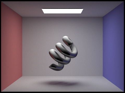
Finally, here are some renders of scenes with a large number of objects:
Direct Illumination refers to the incoming light onto a surface from a light source without indirect bounces. When calculating the illumination an object recieves, we consider the angle of the incoming ray, the bsdf function that describes the surface (ratio/distribution of incoming light to outgoing light), and finally, the actual luminous power and color the ray carries.
Zero-bounce Illumination
In zero-bounce illumination, from a given ray w_in, we would compute the intersection of that ray with our scene. The object that it intersects with gives an emission, which is what I returned from the function.
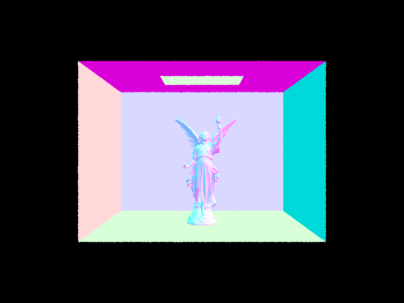
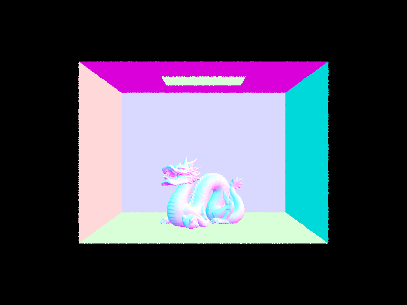
Direct Lighting with Uniform Hemisphere Sampling
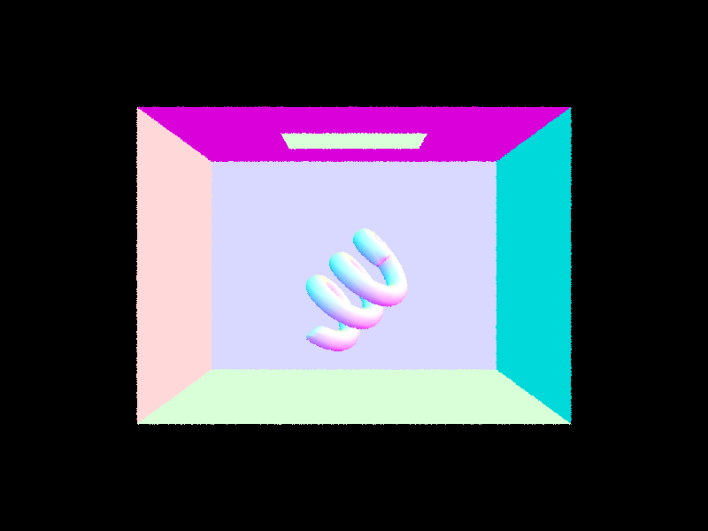
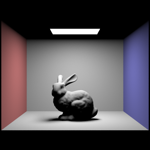
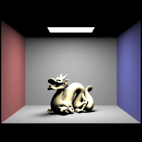
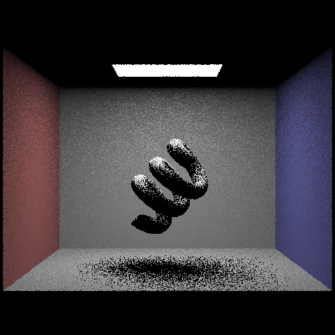
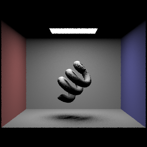
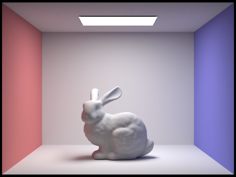
To implement uniform hemisphere sampling for lighting, I sampled for vectors in the hemisphere of the origin point of the ray. Then for each sample, I compute the ray's intersection with the scene, and we can get the illumination by:\begin{equation*}\text{isect.bsdf}\rightarrow\text{get_emission()} \cdot \text{cos_theta(w_in)} \cdot \text{bsdf}\rightarrow\text{f(w_out, w_in)}\end{equation*}Here are some examples:
bunny coil dragon
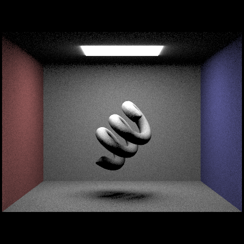
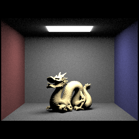
Direct Lighting by Importance Sampling Lights
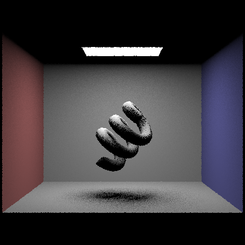
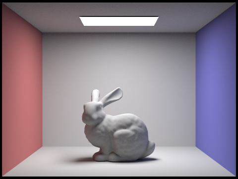
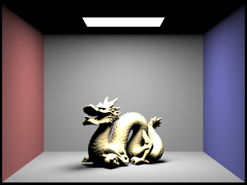
For importance sampling, we iterate over each light and sample from it \(n\) times. After sampling from the light, we set the ray's min_t to EPS_F and max_t to distToLight - EPS_F to check if there are any scene objects between the light and surface that would block the light. If not, we compute the illumination similar to above and take the average out of those \(n\) samples. Since we do not sample uniformly, we need to divide our sample by the probability of making that sample. Finally, summing the illumination over all light sources gives us the lighting from importance sampling.
bunny coil dragon
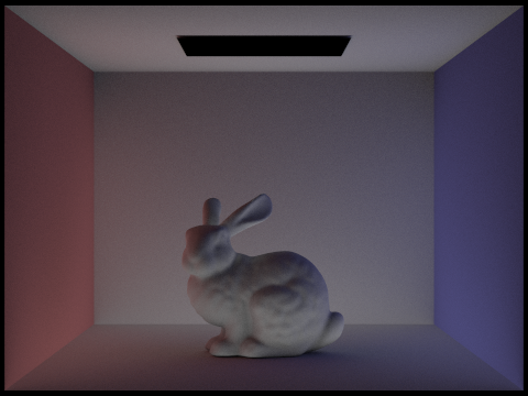
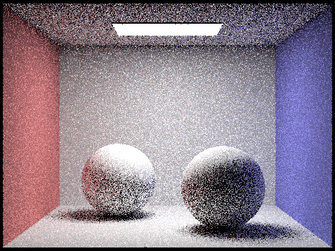
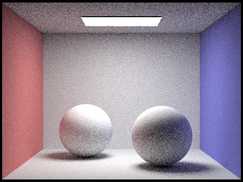
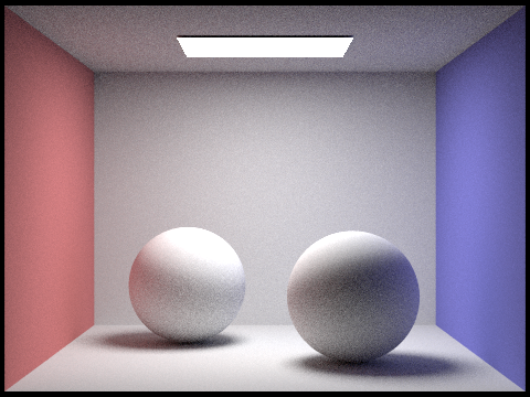
Here is an example of increasing the amount of samples we draw from each light source:
A difference between uniform sampling and importance sampling would be the amount of noise in the image. With importance sampling, we sample directly from the light source, which allows us to converge faster to the solution. From the images above, the ones obtained from uniform sampling are grainier, with much more variation in the color on each wall compared to importance sampling.
Global Illumination
For indirect lighting, we would use a recursive function and trace a ray to a surface. If the ray's depth was 1, we would just return the one bounce illumination from the previous part. Otherwise, we sample a ray on the hemisphere, translated to world coordinates, recurse using the function. Since the function returns incoming light, we would multiply by the bsdf and cos_theta for the angle, giving the illumination of the surface.
This is the illumination where we do not accumulate the illumination from previous bounces:
When the light is not accumulated, with more bounces, it loses brightness, and this makes sense because the light is scattered when it comes in contact with a surface. When the light is accumulated, the scene becomes brighter, because many areas are more likely to come in contact with light rays when we allow for more bounces.
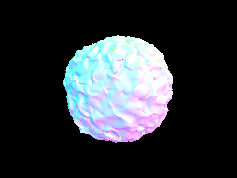
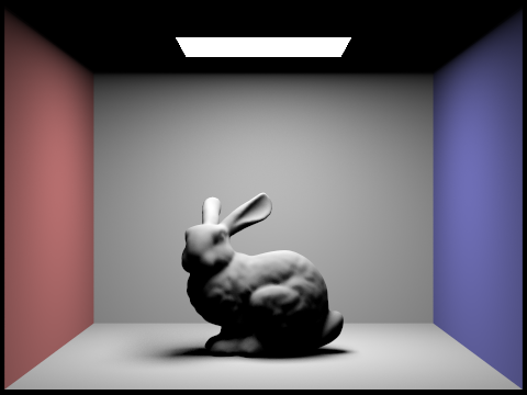
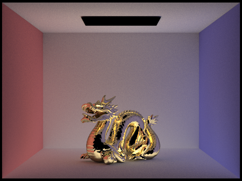
We can also split the rendering into direct and indirect lighting. Something interesting to note is that with direct lighting, we get the base color of the object while indirect lighting captures more of the reflective properties of the object:
original direct indirect
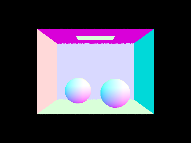
Finally, this shows spheres rendered with a varying number of samples-per-pixel:
1 spp 2 spp 4 spp 8 spp 16 spp 64 spp 1024 spp
Russian Roulette
Computing the global illumination requires us to sum over all the \(k\)-bounces of light through a scene for \(k \geq 0\). An unbiased solution to this problem involves flipping a coin with weight \(cpdf\) to check whether the ray should continue bouncing. If it does, we calculate the incoming light and divide that additionally by the \(cpdf\). If not, we return the one bounce illumination function as the base case.
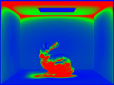
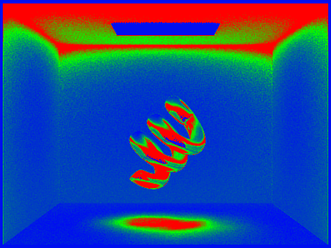
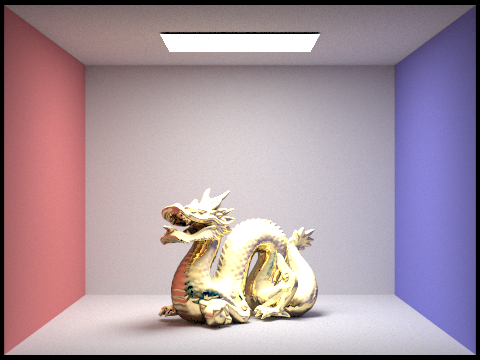
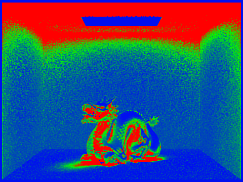
In adaptive sampling, we check that the margin of error is less than a given tolerance. So given \(n\) samples, I calculated the illumination of the sample, the average illumination and variance of illumination. Then \begin{equation*}I = 1.96 \cdot \sqrt{\frac{\sigma^2}{n}}\end{equation*}and I checked for every \(32\) samples if \(I \leq maxTolerance \cdot \mu \) which would be the condition to stop. Here are some results:
bunny S=2048 M=5 bunny sampling rate
coil S=2048 M=5 coil sampling rate
dragon S=2048 M=5 dragon sampling rate
With adaptive sampling, parts of the scene that are not directly visible to the light are sampled more. For instance, the shadow of the bunny and coil are red, while the walls are blue.