In this assignment, I learned about how the mass, spring equations can be used to model structural, shearing, and bending forces on a cloth. Two interesting things was how we can hash a given point into a bin given a subdivision of the space, as an alternative to using a bvh to find collisions, and how shaders can be used to add texture to objects.
Masses and Springs
For the implementation, I did a double for loop over the number of points along the width and height. Then we can do a bounds check to see if we can add a spring corresponding to the given forces:
The structural forces on the cloth are given as a spring from a point mass to the point mass above as well as one to the left.
The shearing forces on the cloth are given as a spring from a point mass to the upper left and upper right.
The bending forces on the cloth are given as a spring from a point mass to the point mass two above as well as one two away on the left.
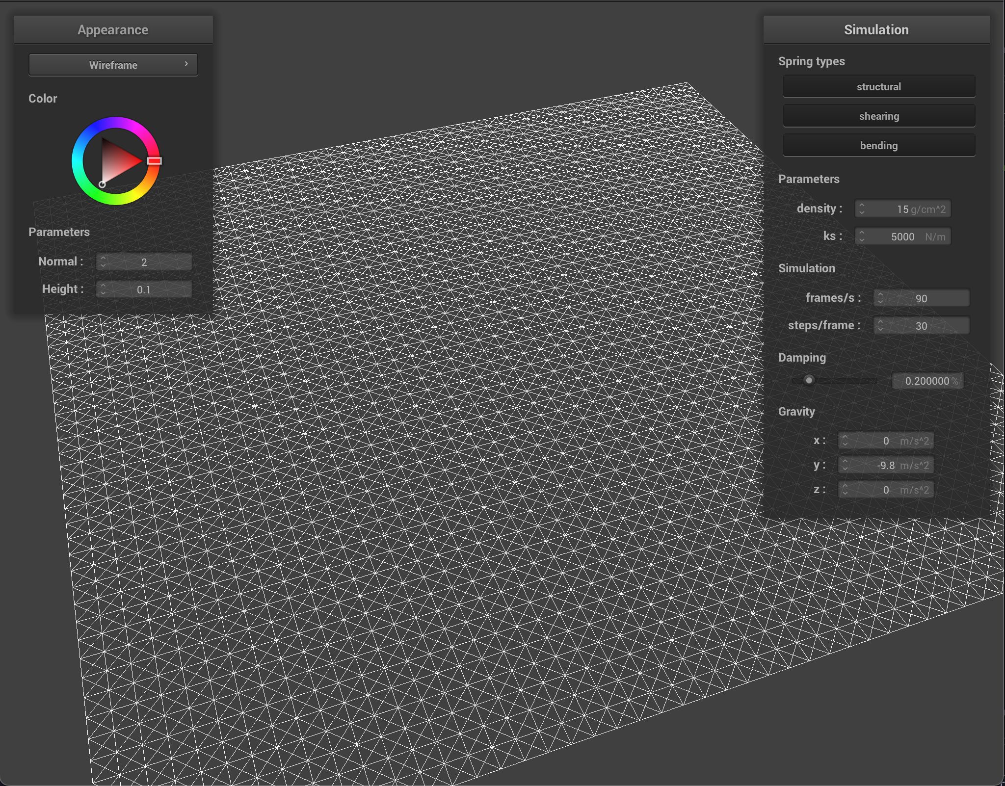
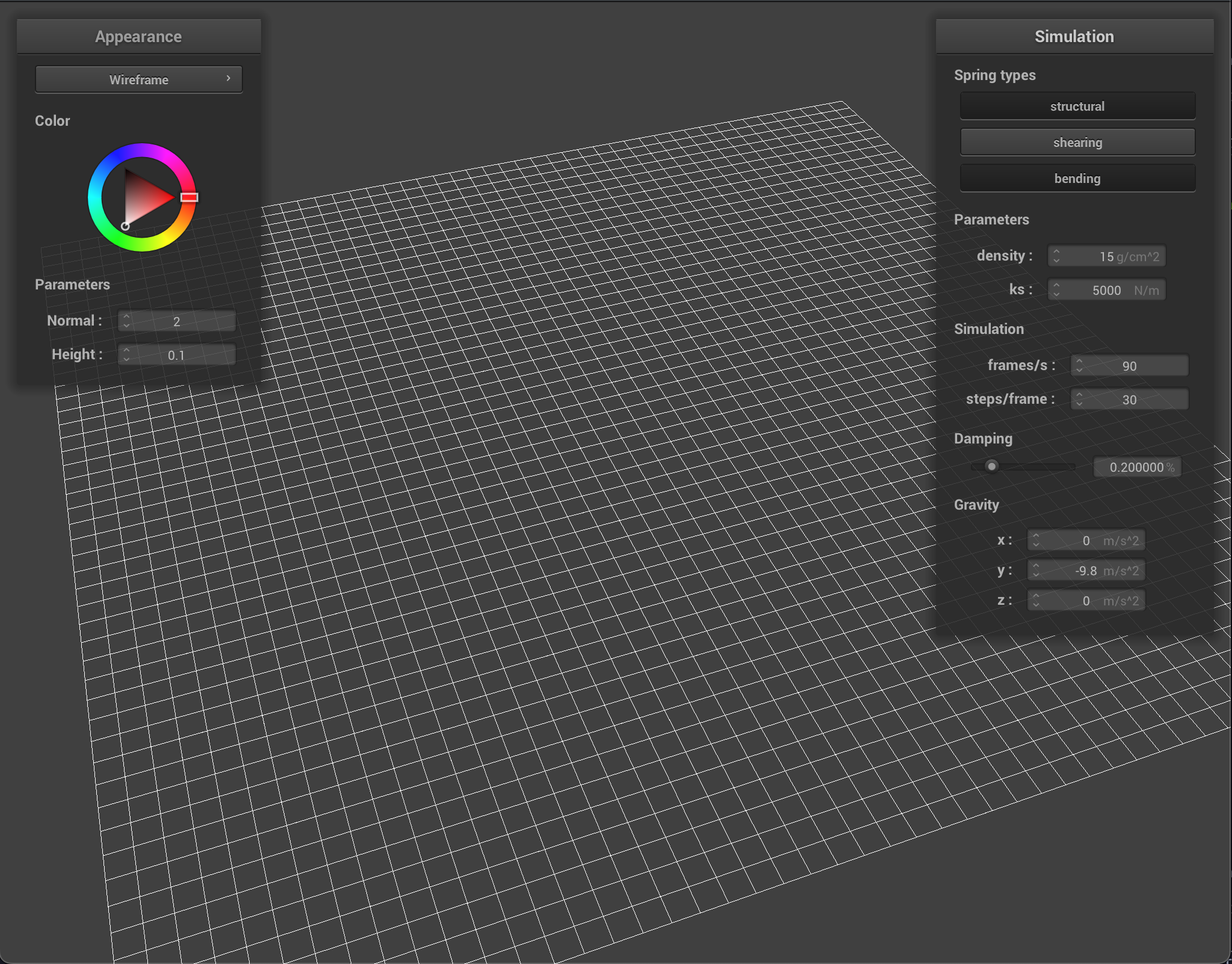
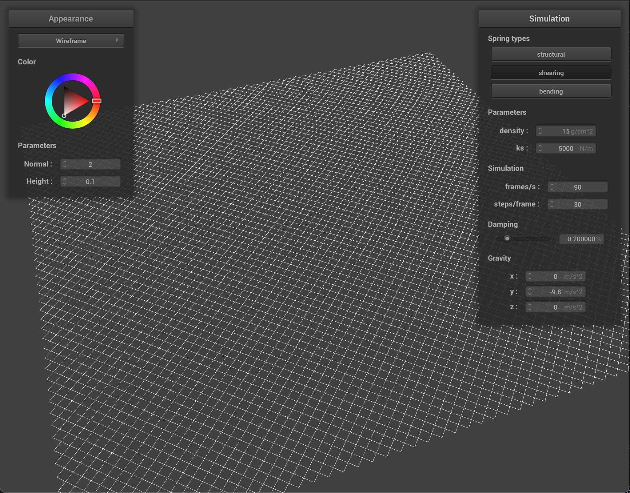
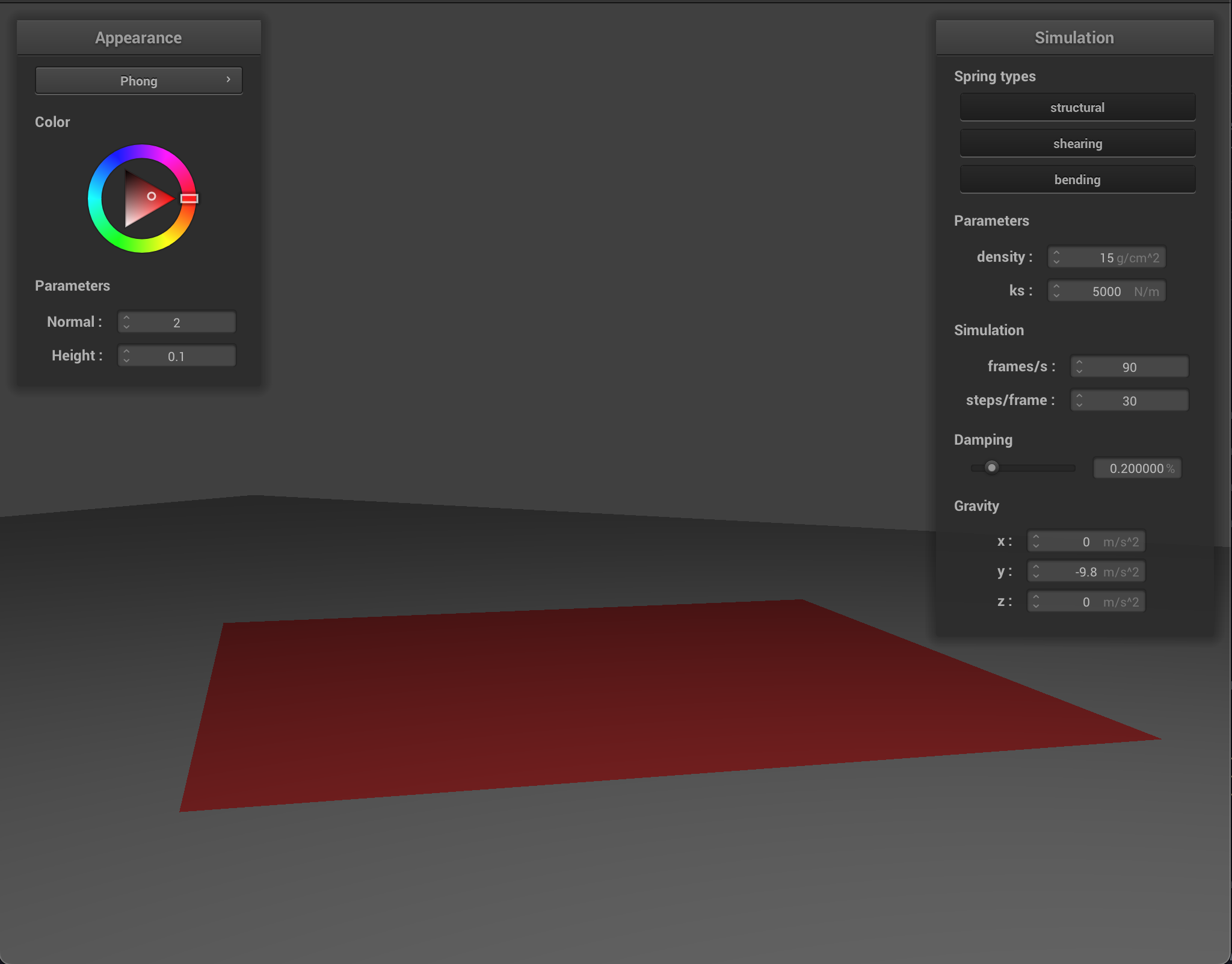
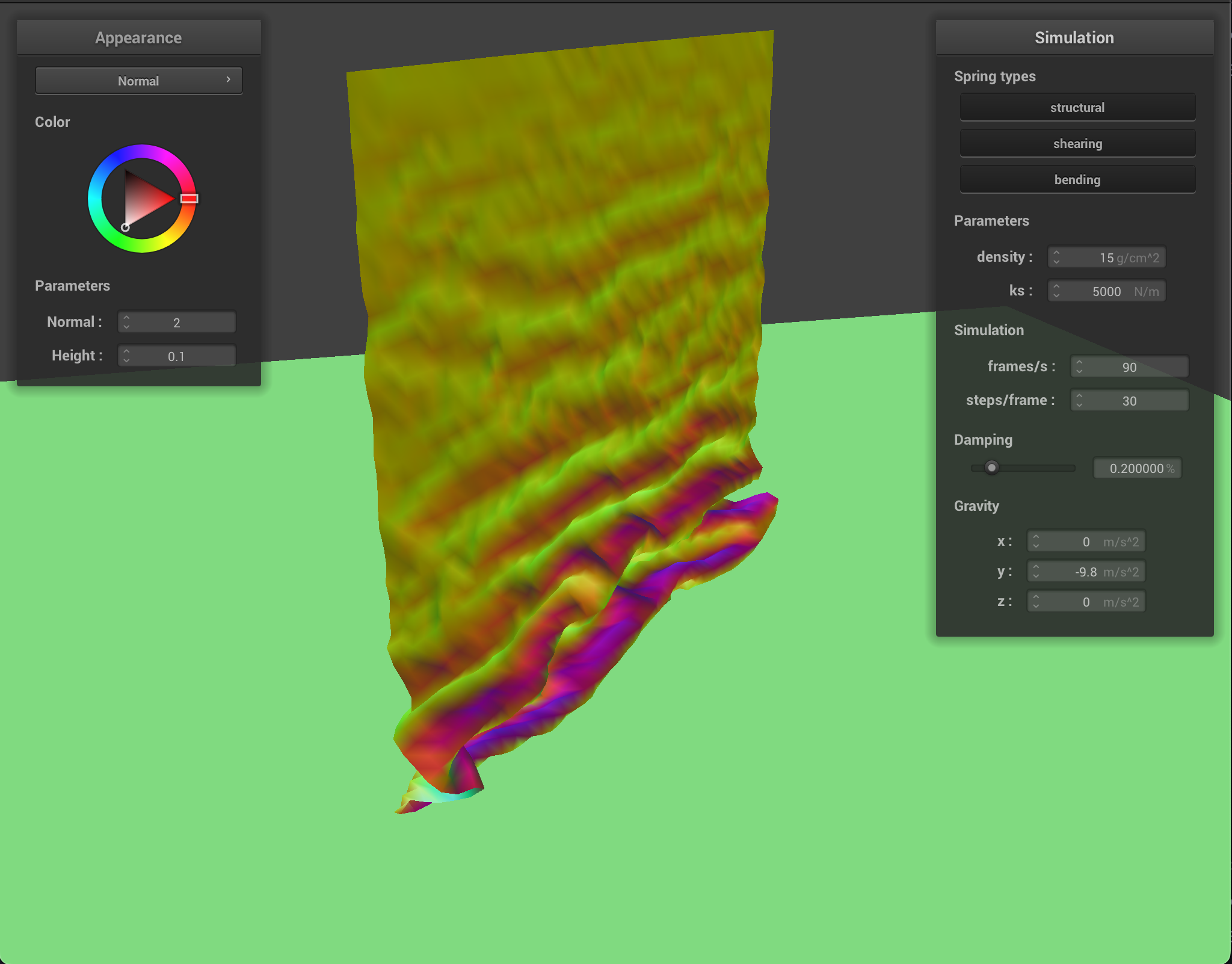
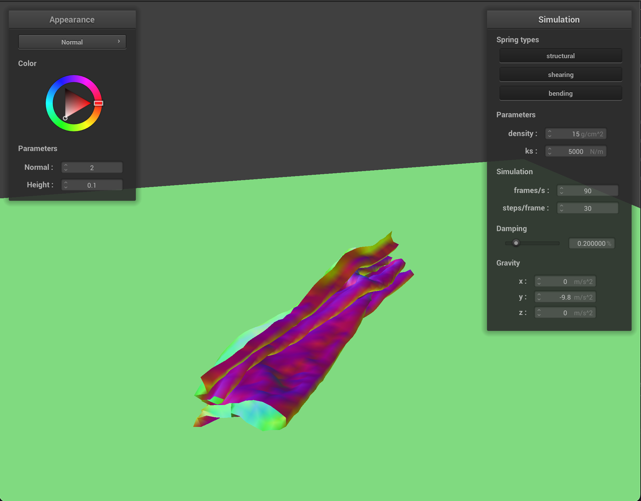
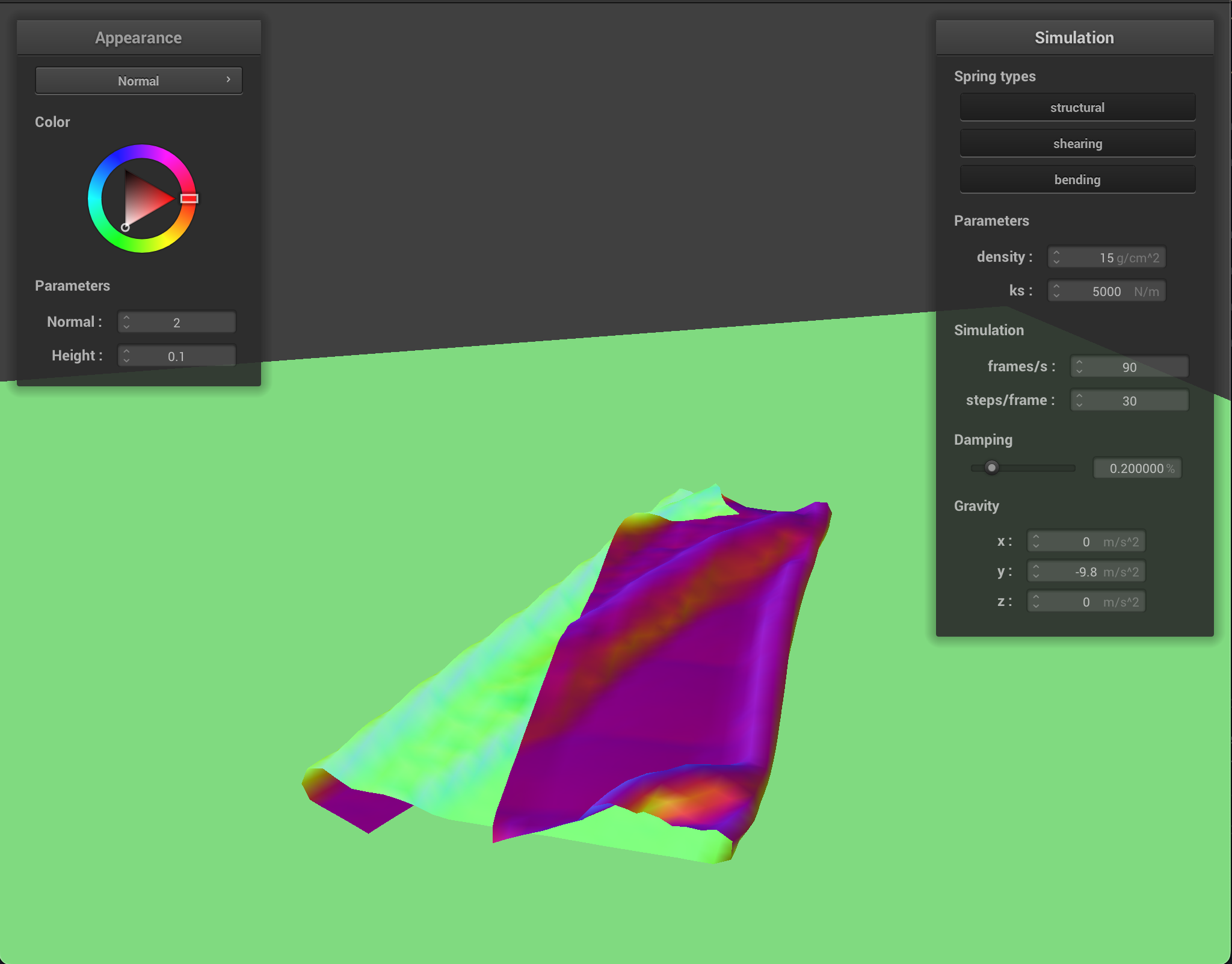
For the following images, st represents structural springs, sh for shearing, and bd for bending:
Spring types: st+sh+bd Spring types: st+bd Spring types: sh
Simulation
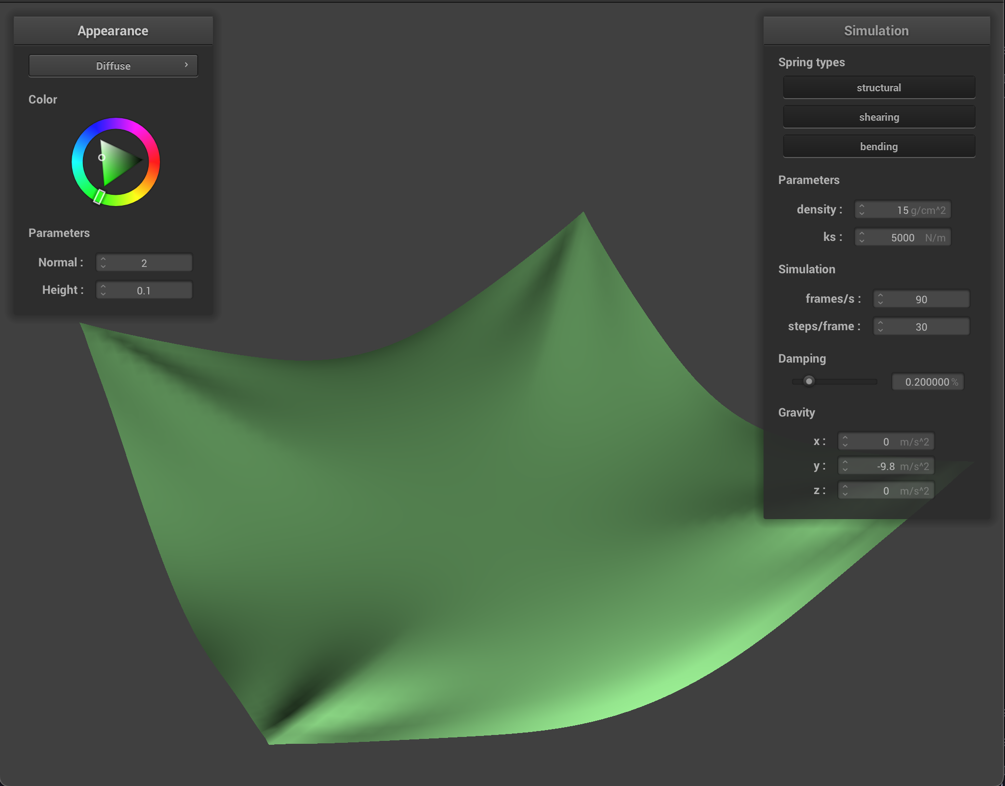
To simulate the forces on the cloth, we first initialize the total force on each point mass to be the sum of\(F = m \cdot a\) where \(a\) is a given acceleration in a list of external accelerations. Next, we loop over each spring, and calculate the magnitude of the force:\begin{equation*} F_{s} = k_{s} \cdot (\lVert p_{a} - p_{b} \rVert - l) \end{equation*} Then the force of the spring on \(p_{a}\) would be a vector in the direction of \(p_{b}\) of magnitude \(F_s\).
Here is what the cloth looks like when we add these forces:
Cloth pinned at 4 cornersCloth pinned at 2 corners
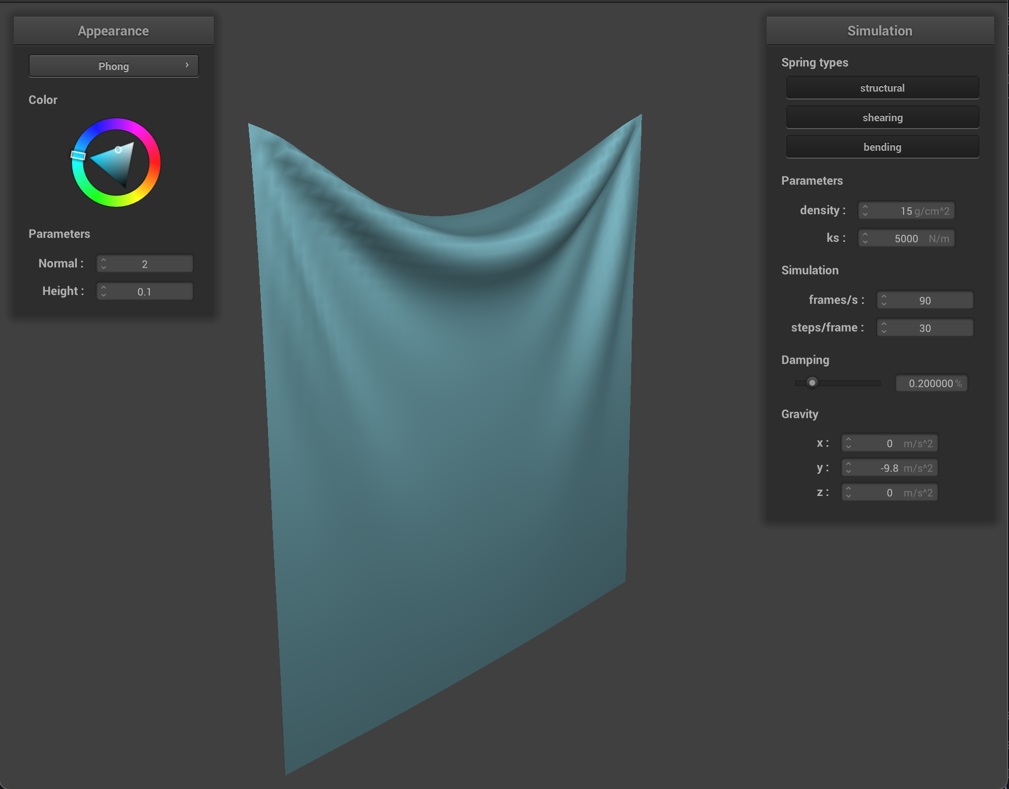
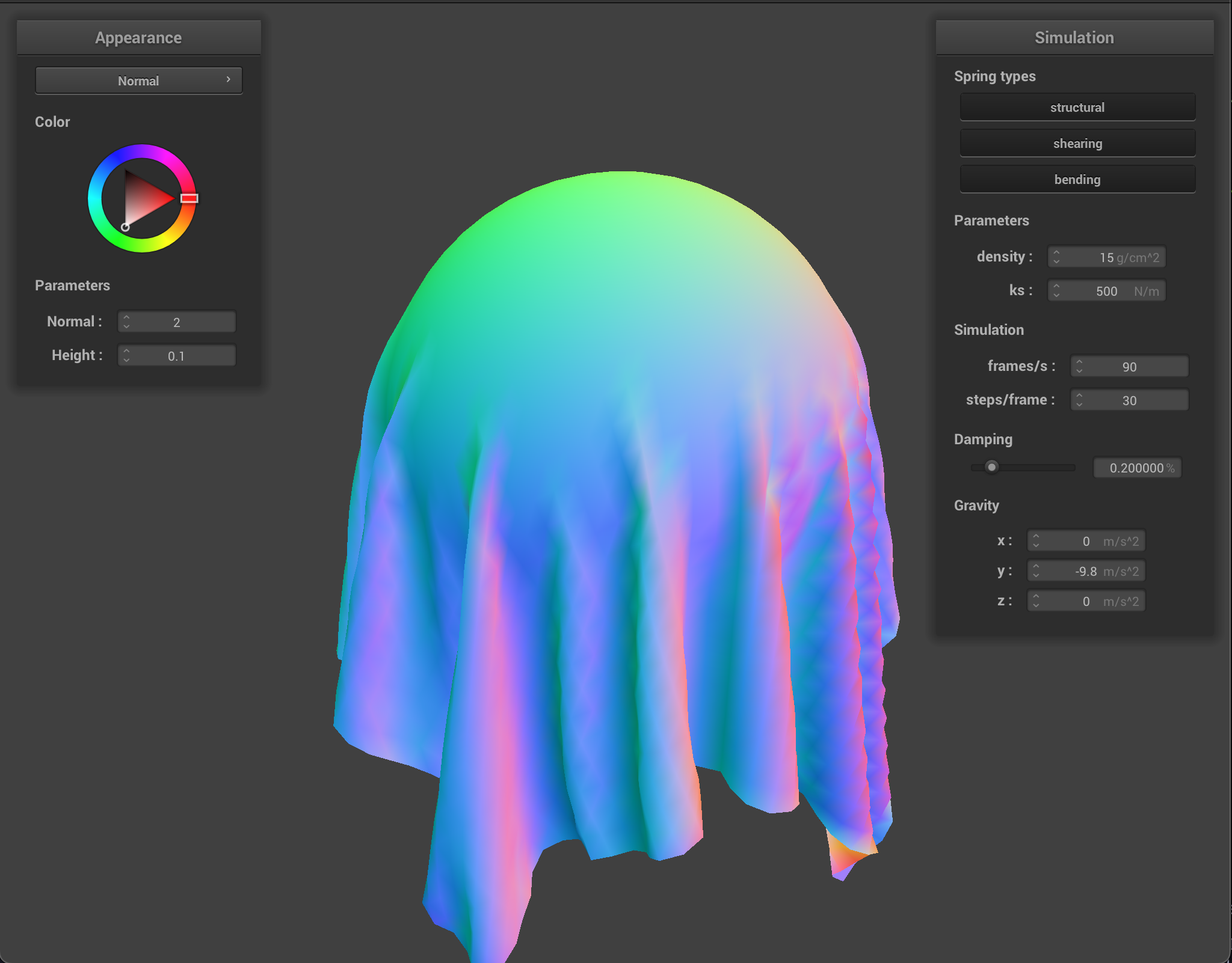
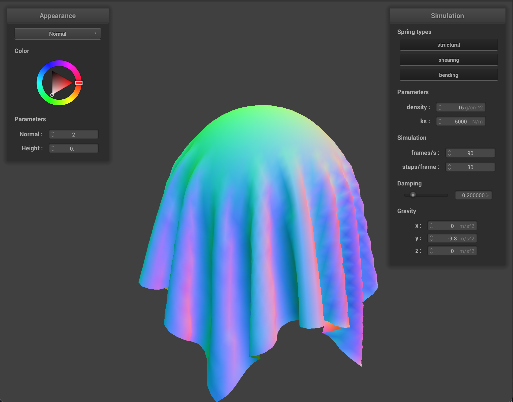
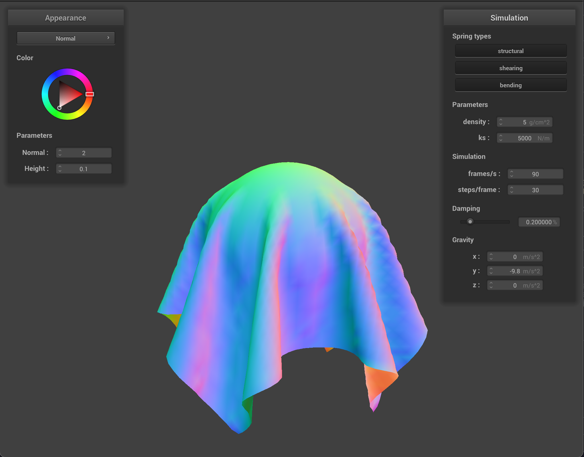
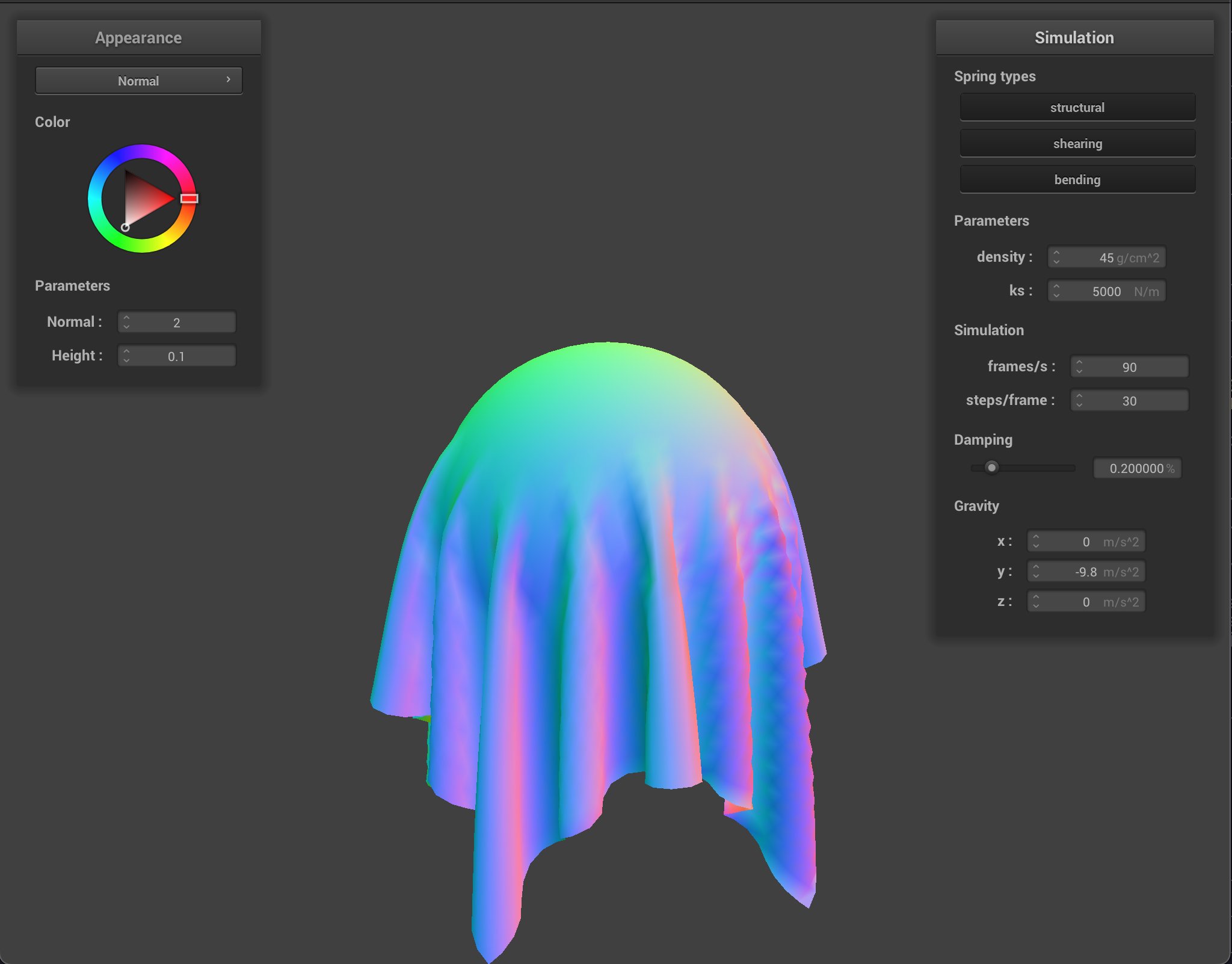
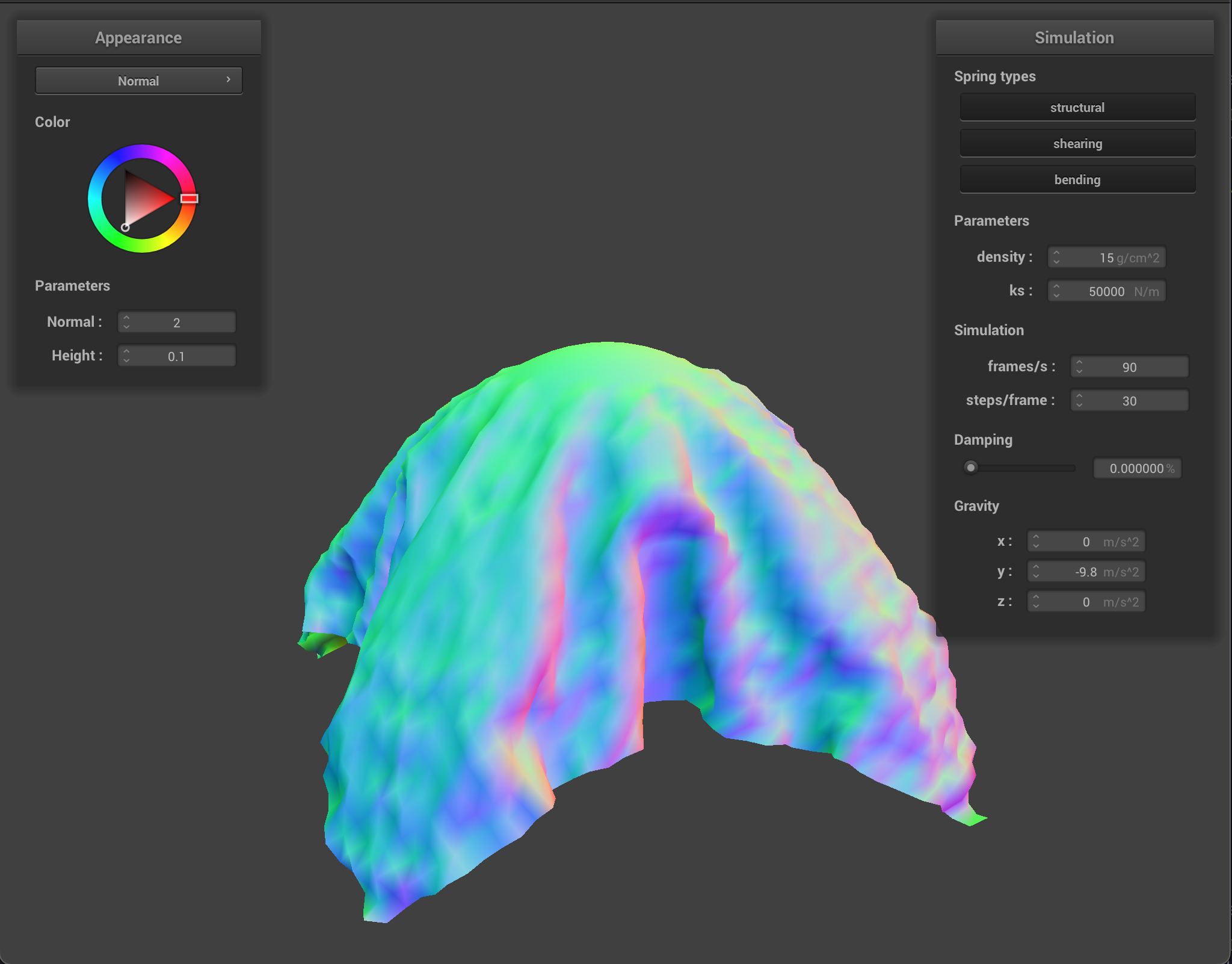
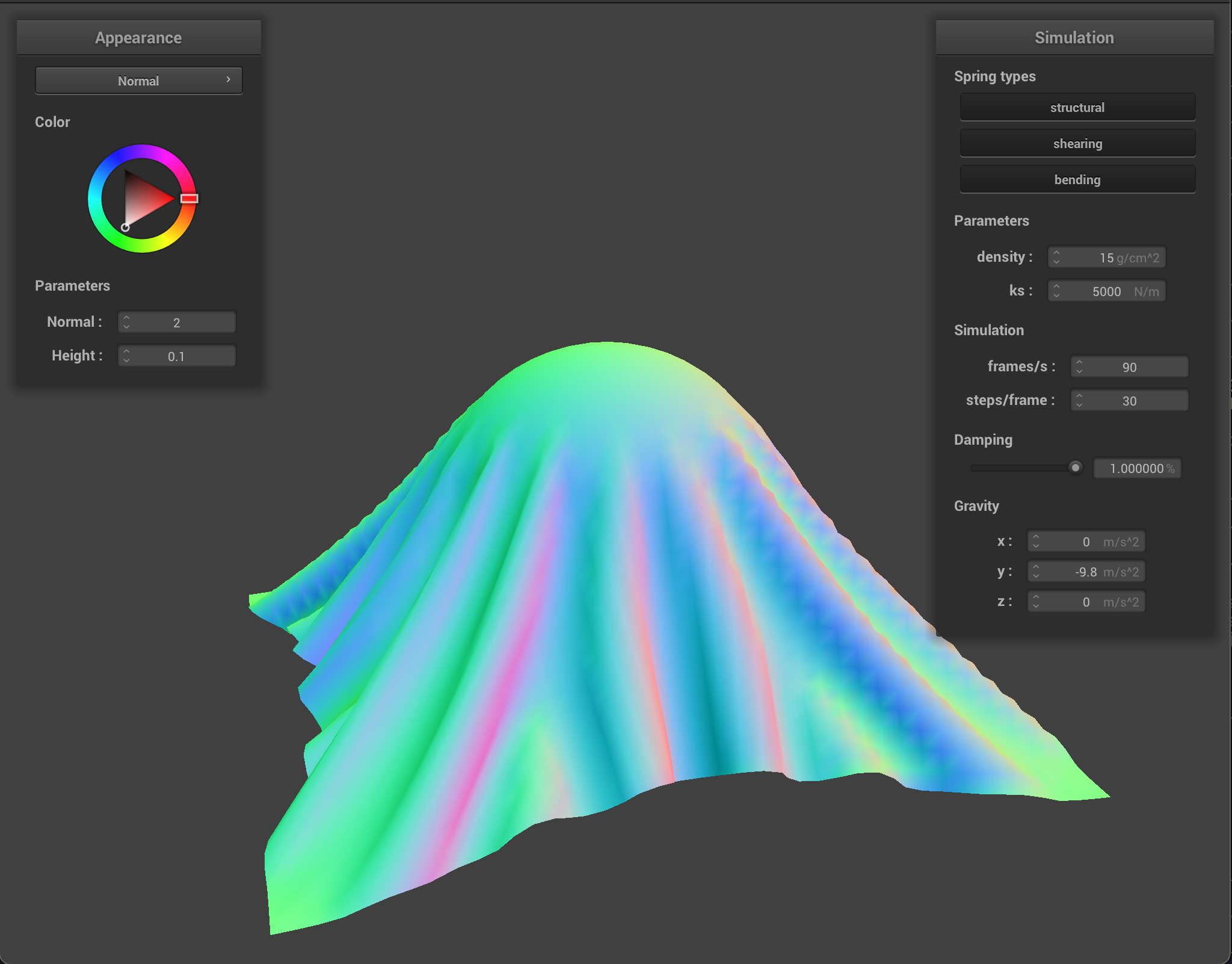
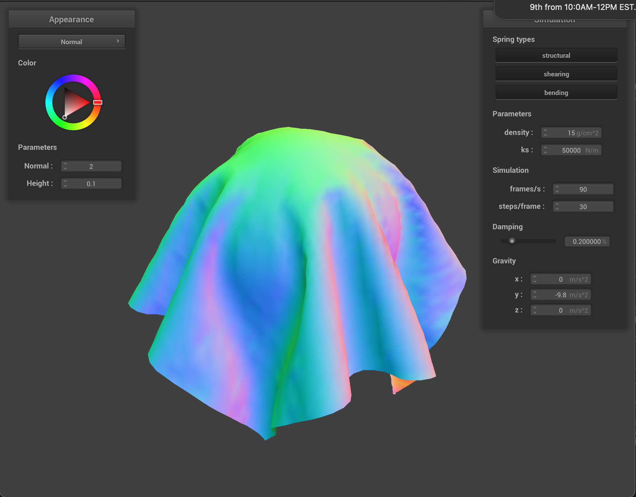
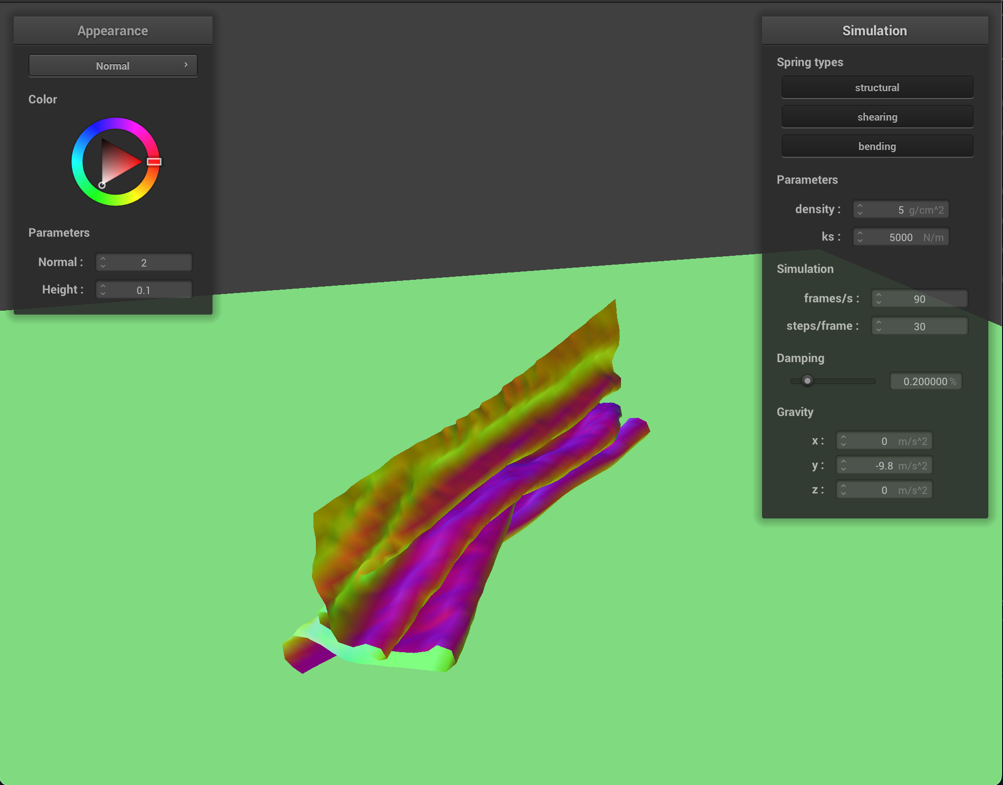
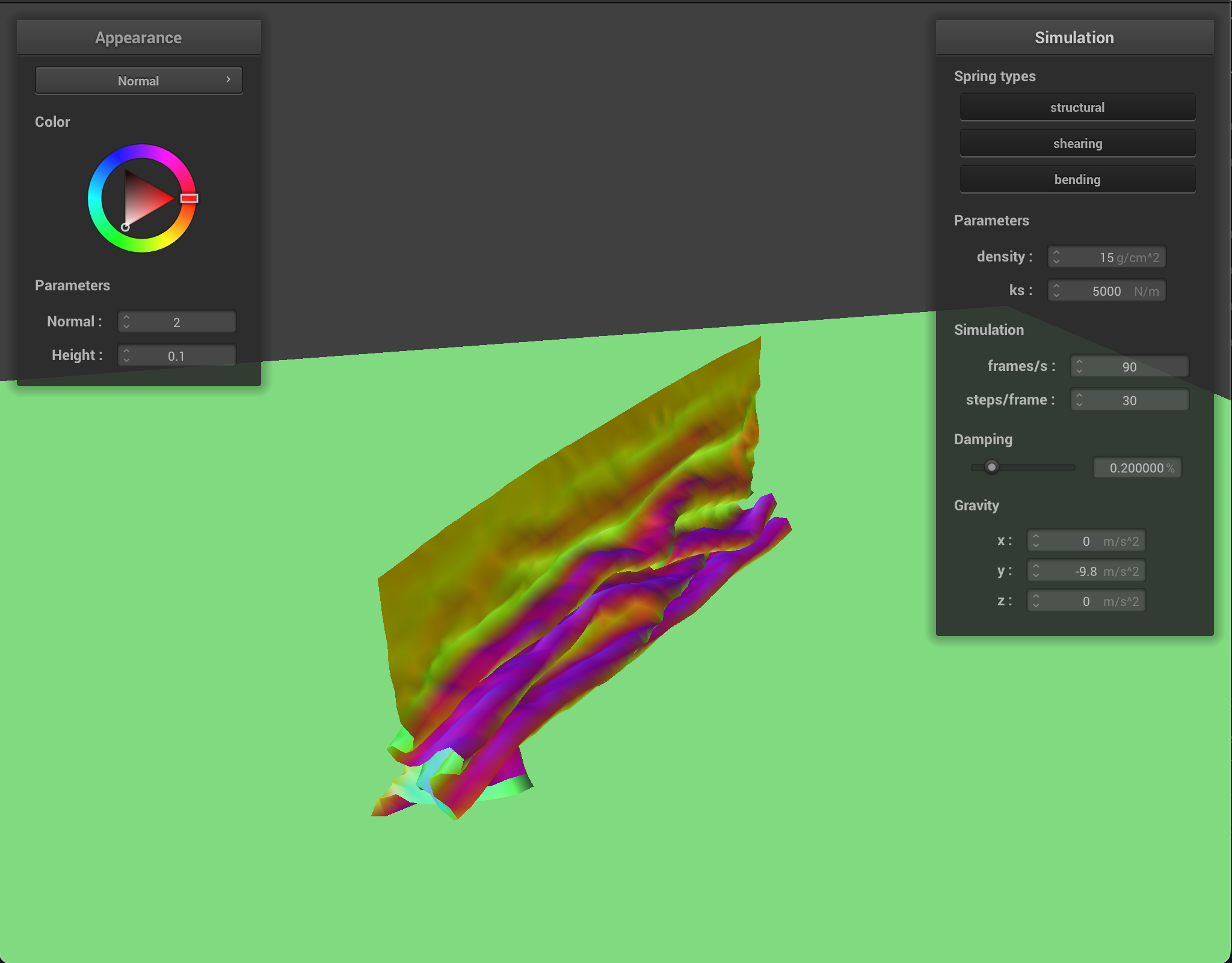
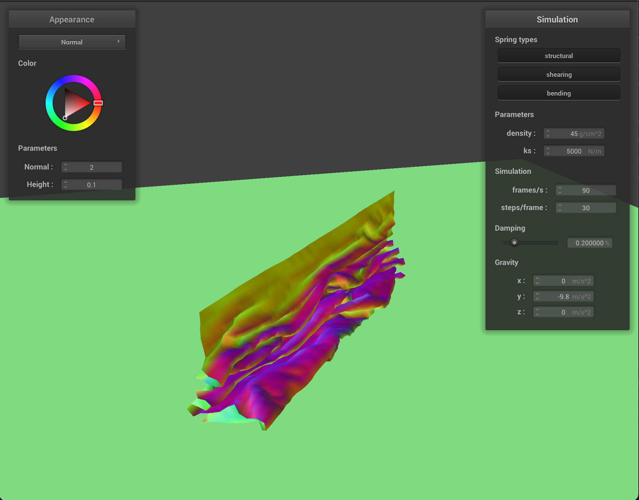
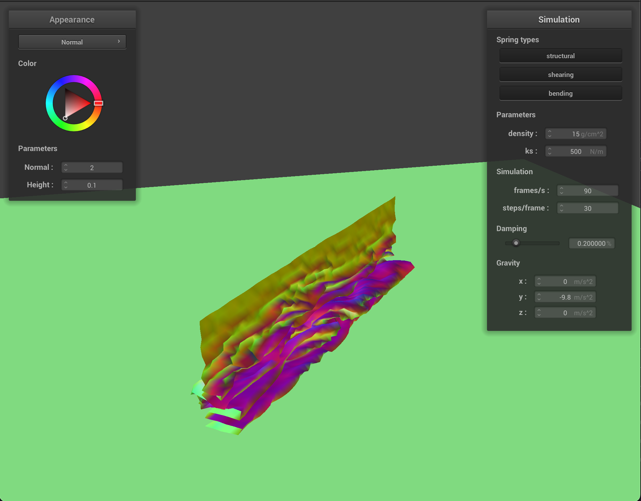
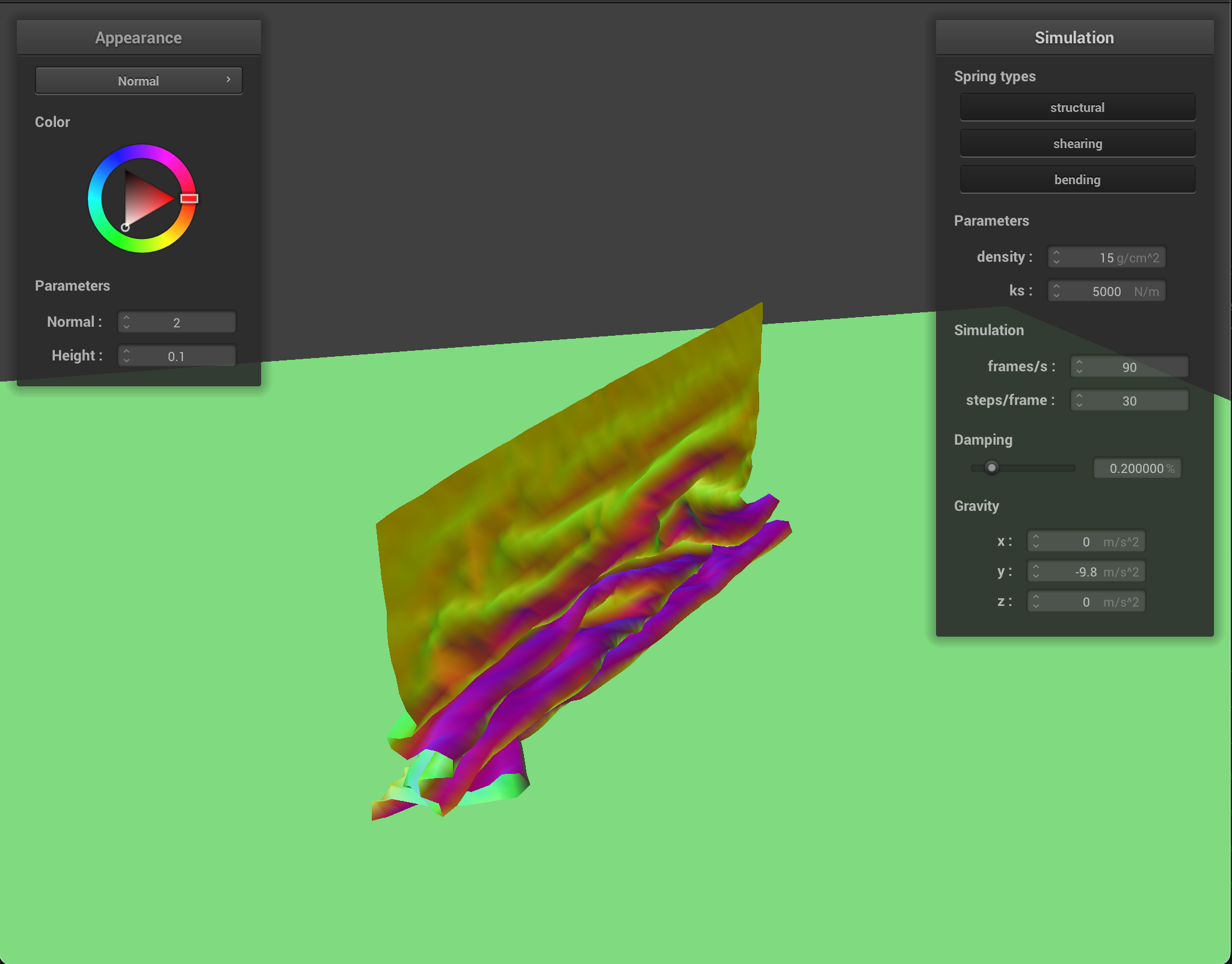
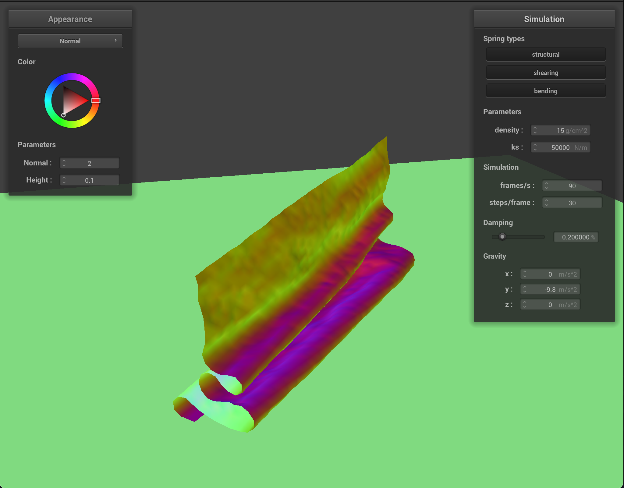
The following images illustrate how varying the parameters of the cloth can affect the cloth:
\(K_s\)= 500, Density = 15 \(\frac{g}{m^2}\), Damping = .2%\(K_s\)= 5000, Density = 15 \(\frac{g}{m^2}\), Damping = .2%\(K_s\)= 50000, Density = 15 \(\frac{g}{m^2}\), Damping = .2%\(K_s\)= 5000, Density = 5 \(\frac{g}{m^2}\), Damping = .2%\(K_s\)= 5000, Density = 15 \(\frac{g}{m^2}\), Damping = .2%\(K_s\)= 5000, Density = 45 \(\frac{g}{m^2}\), Damping = .2%\(K_s\)= 5000, Density = 15 \(\frac{g}{m^2}\), Damping = .0%\(K_s\)= 5000, Density = 15 \(\frac{g}{m^2}\), Damping = .2%\(K_s\)= 5000, Density = 15 \(\frac{g}{m^2}\), Damping = 1%
I noticed that as the spring constant increases, the cloth became stiffer where a spring constant of \(50000\) made the cloth resistant to folding. A higher density had a similar but inverse effect. Finally, decreasing the damping of the cloth made the collision with the sphere stronger. For the change in damping, the images were captured as the edges of the cloth were falling, and in the low damping picture, the cloth springs back up while for high damping, the cloth drapes down softly.
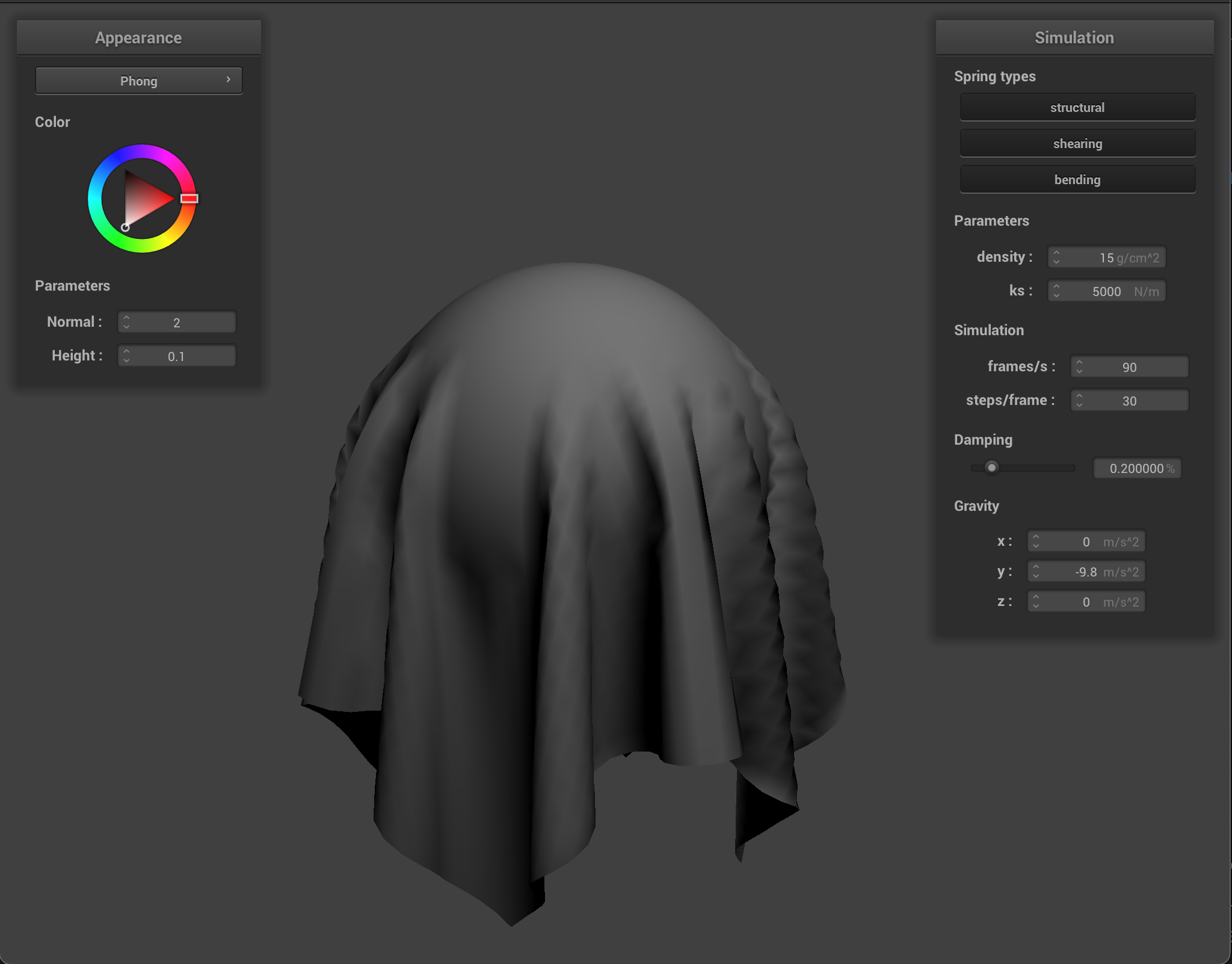
Collisions with Spheres and Planes
For collisions with spheres, we calculate if the new position of the point mass is within the radius distance from the sphere's origin. If the new position is inside the sphere, we move along the origin-point mass ray to bump the position to the surface of the sphere. Adding in friction, this corrects the position of the point mass.
\(K_s\) = 500\(K_s\) = 5000\(K_s\) = 50000
From the images, a higher spring constant makes the cloth stiffer and more resistant to folding. This makes sense as a higher spring constant means the spring pulls the point masses together with greater force.
For collisions with a plane, we check if the new position of the point mass is on the same side as that of the last position of the point mass. This is done using the check that: \begin{equation*} (pm.pos - plane.p) \cdot n * (pm.lastpos - plane.p) \cdot n <= 0 \end{equation*} If the path intersects the plane object, we calculate the intersection which becomes the corrected position of the point mass.
Self Collisions
We would only need to correct for collision of the cloth with itself if the point mass is within \(2 \cdot thickness\) where \(thickness\) is the thickness of the cloth. In fixing the position at the collision, we would move along the ray joining the two point masses and set the new position of the point to be \(2 \cdot thickness\) away from the other point mass.
Time: startTime: midTime: end
Varying the density of the cloth, a higher density tends to the leave the bottom of the cloth more scrunched up with the plane:
As for the spring constant, a higher spring constant makes the cloth more resistant to wrinkling:
\(K_s\): 500\(K_s\): 5000\(K_s\): 50000
Shaders
Shaders run parallel to the simulation program and are composed of two parts called the vertex shader and fragment shader. The vertex shader modifies the normals and position of a vertex to set its final position and as input for the fragment shader. The fragment shader computes the color at a vertex to get the final color. The output of both are interpolated in the mesh to color the object.
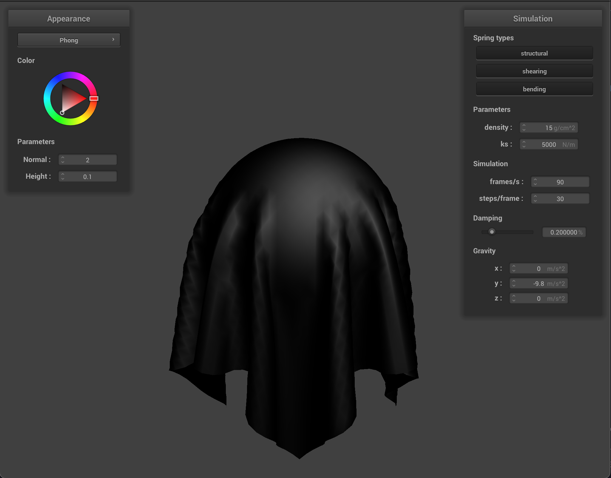
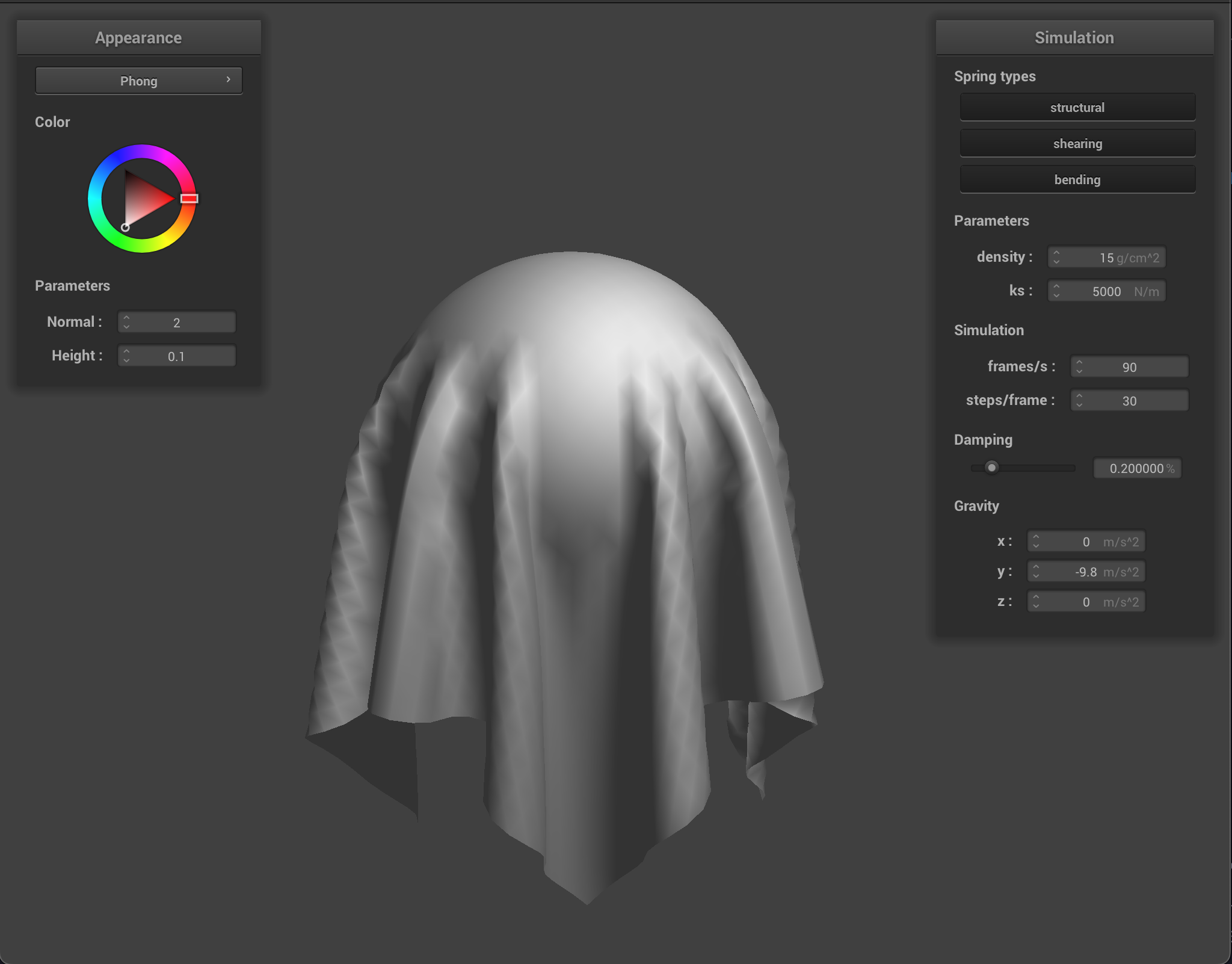
Blinn-Phong Shading
In Blinn-Phong Shading, there are three components: diffuse lighting, ambient lighting, and specular highlights. Ambient lighting is given by the base color of the object:\begin{equation*} L_a = c \cdot k_s \cdot I_a \end{equation*}Diffuse lighting is given by the luminance from the object as a function of the light position and the angle of the surface:\begin{equation*} L_d = c \cdot k_d (I / r^2) \max{n \cdot l, 0} \end{equation*}Where \(l\) is the unit vector in the direction of light from the surface point. Finally, specular highlights are given by:\begin{equation*} L_s = c \cdot k_s (I / r^2) \max{n \cdot h, 0}^p\end{equation*}
Lighting: ambientLighting: diffuseLighting: specularLighting: all
For the ambient lighting, I used the values: \(k_a = 1., I_a = (.2, .2, .2)\). For diffuse lighting, I used \(k_d = .7\), and finally, for specular, I used \(k_s = .5, p = 5\).
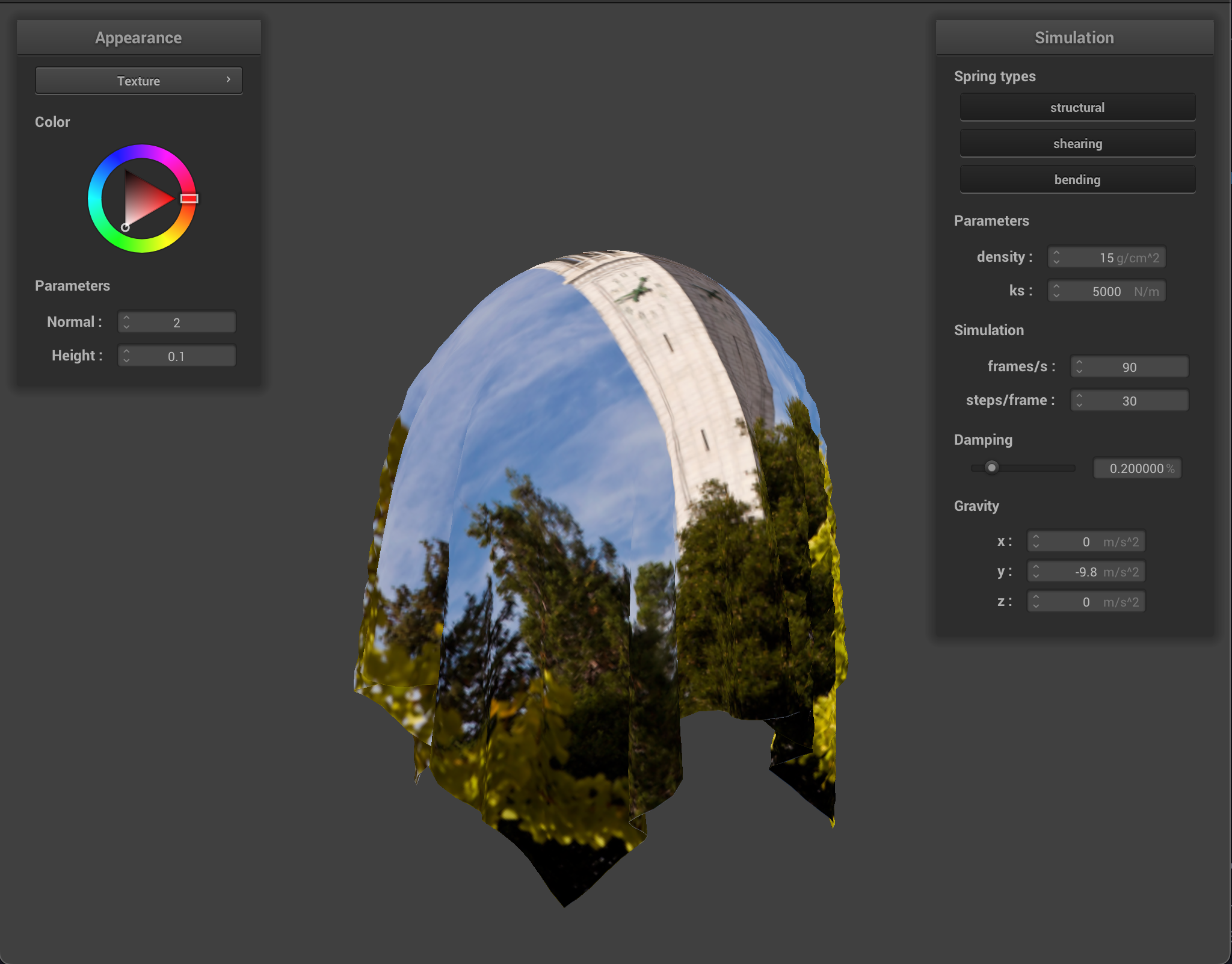
Texture Mapping
For the texture mapping, we are given a \(uv\)-coordinate in the frag file and can call the texture function to sample from the texture. The output of this function is the color of the vertex.
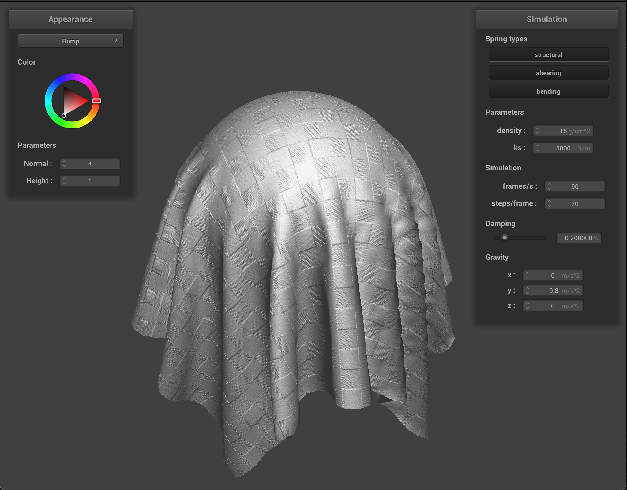
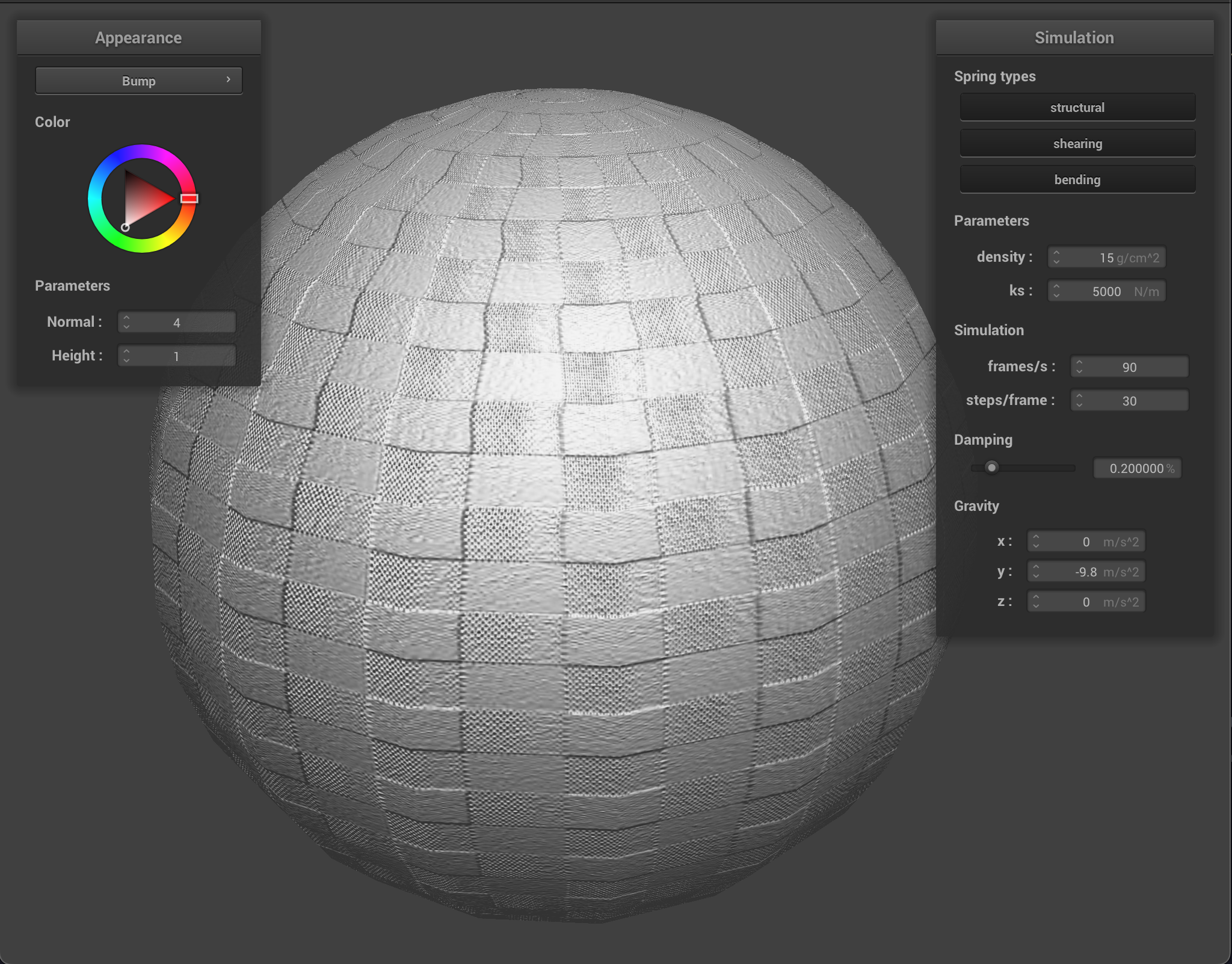
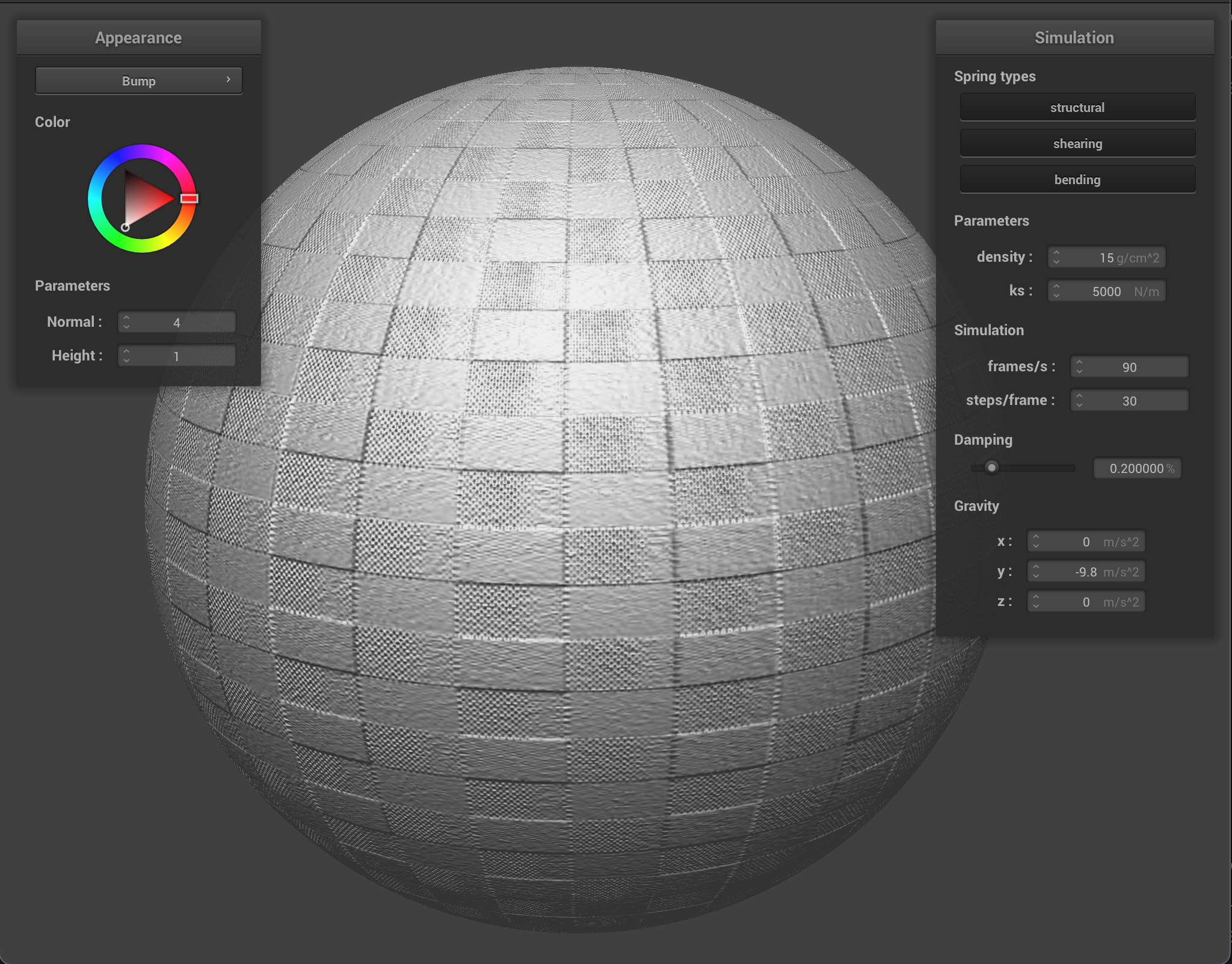
Bump Mapping
In bump mapping, we compute the height of a vertex by a function given the \(uv\)-coordinates \(h(u, v)\). To recompute the normal of the vertex given the height, we compute the change in height wrt to \(du, dv\) given as:\begin{align*} dU &= (h(u + 1 / w, v) - h(u, v)) \cdot k_{h} \cdot h_{k} \\ dV &= (h(u, v + 1 / h) - h(u, v)) \cdot k_{h} \cdot k_{n} \end{align*} Where \(k_h, k_n\) are scaling factors for the height and normal respectively. The modified normal is given by a linear combination of the tangent, bitangent, and normal vector to the vertex:\begin{equation*} \begin{bmatrix} \mid & \mid & \mid \\ \vec{T} & \vec{B} & \vec{N} \\ \mid & \mid & \mid \end{bmatrix} \begin{bmatrix} -dU \\ -dV \\ 1 \end{bmatrix} \end{equation*} In the following simulation, I used the fourth texture from the given texture folder
Bump coarseness: 16Bump coarseness: 128
From the images above, a lower coarseness makes the bump mapping less jagged and more consistent. In the picture where the coarseness is set to 16, the surface of the sphere is not as smooth, so the bump mapping gets messed up.
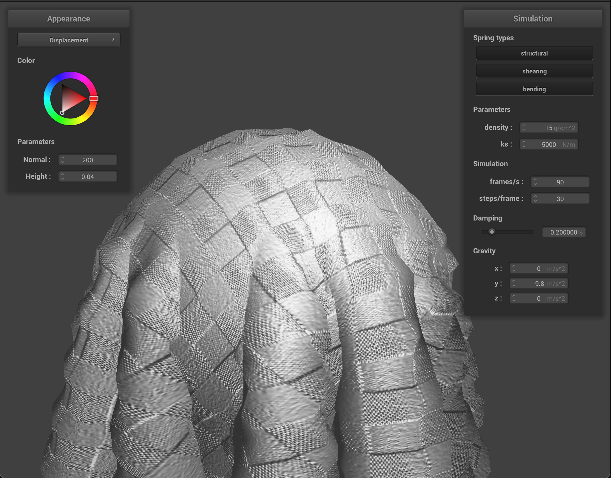
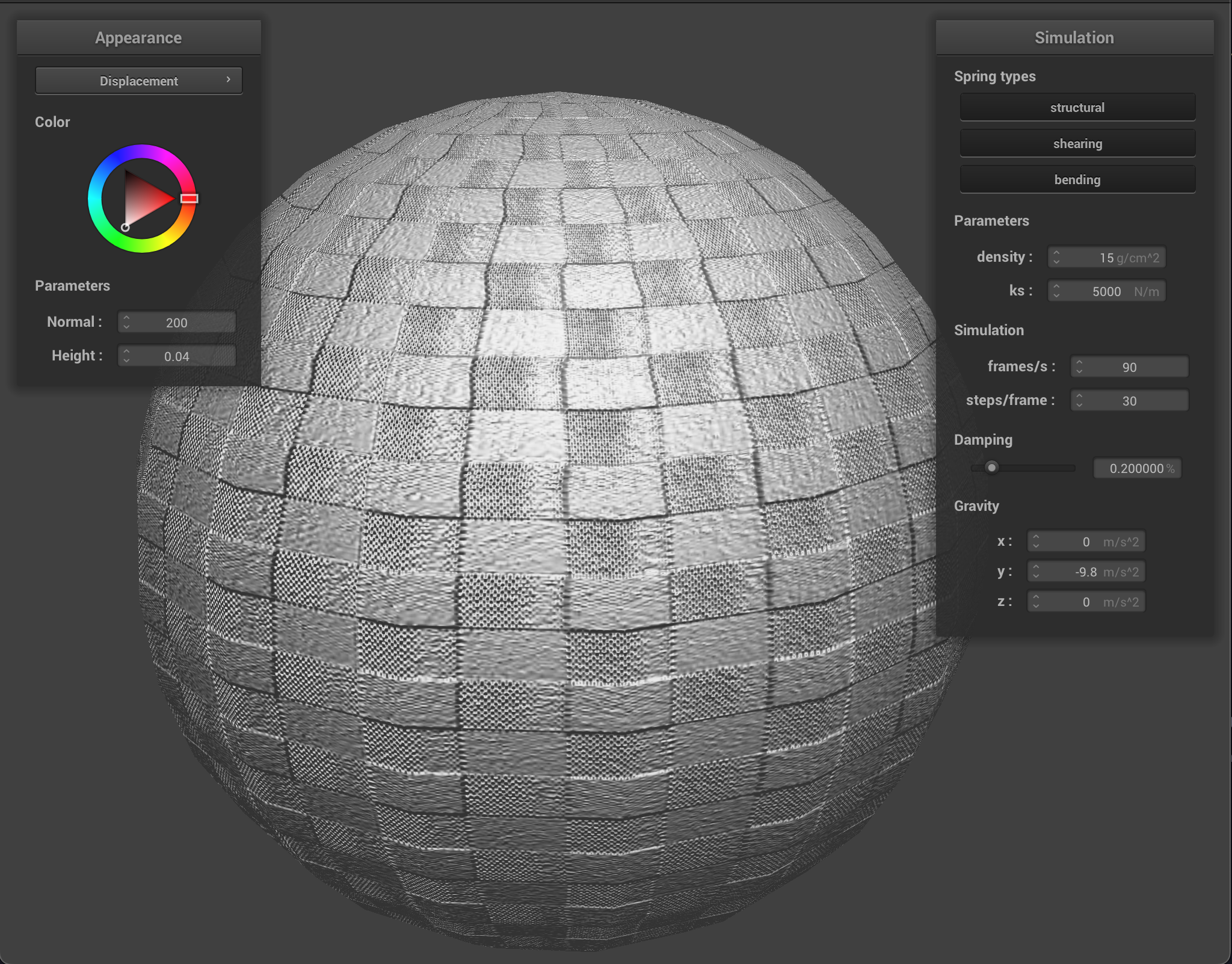
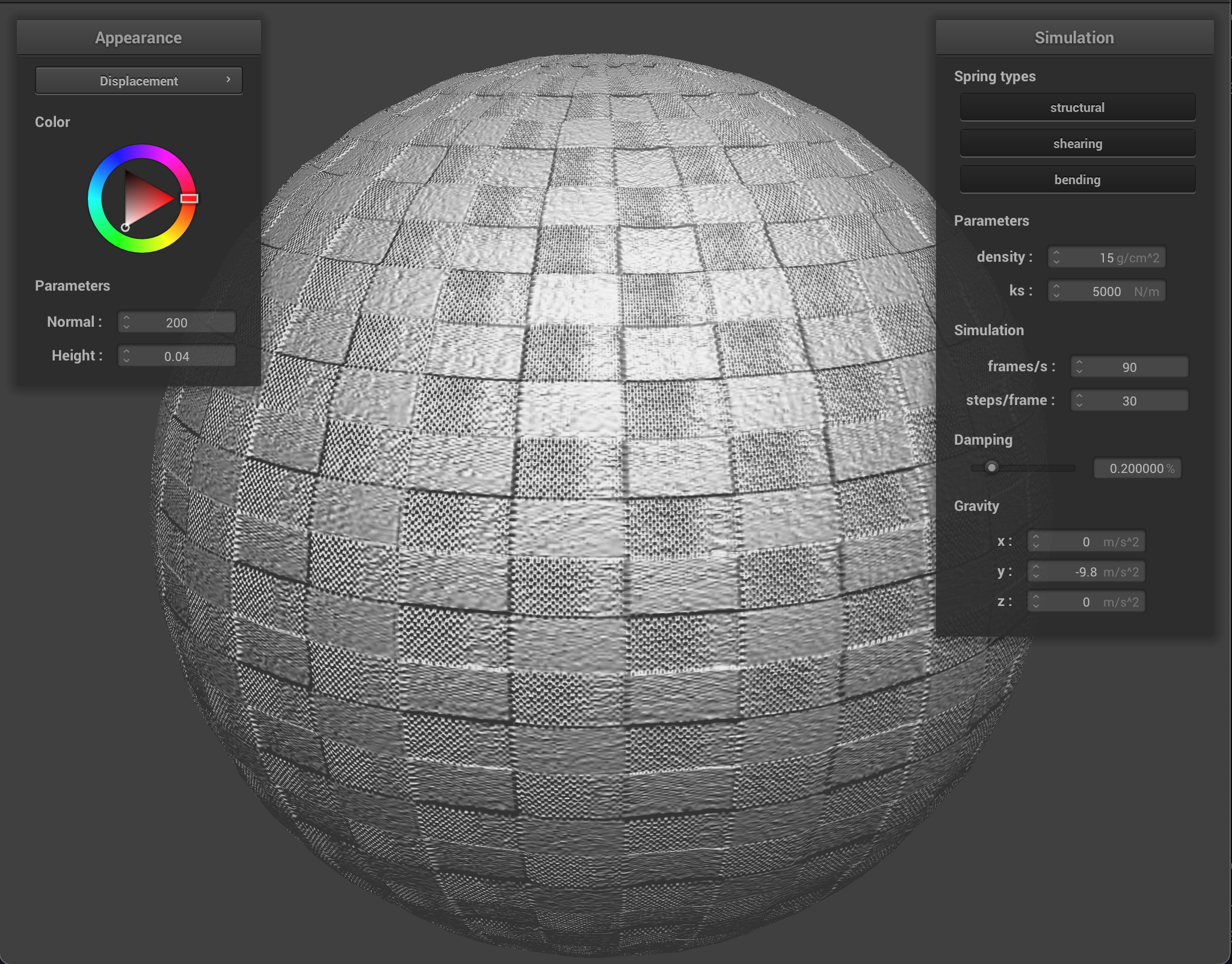
Displacement Mapping
Displacement mapping adds on to bump mapping in that we modify the vertex' position by the recomputed normal. The new position is given by:\begin{equation*} p^{\prime} = p + n \cdot h(u, v) \cdot k_{h} \end{equation*}In the following simulation, I used the fourth texture from the given texture folder
Here is an adjustment of the coarseness of the sphere mesh:
For the sphere mesh on the right with more points, the indentation on the sphere at certain squares is more visible, and we can see this when looking at the silhouette of the sphere. With the more coarse mesh, the indentation is lost and the surface is less detailed. Hover over the images to zoom-in.
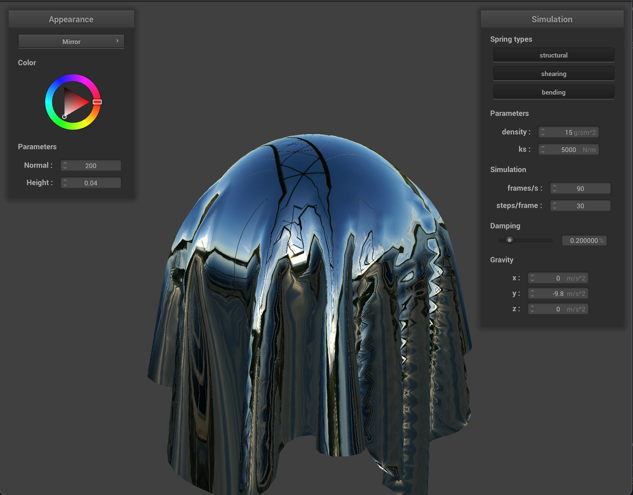
Bump/Displacement Mapping Comparison
I would say that bump mapping is more effective than displacement mapping for applying texture, because the vertex positions are not very consistent with the height map. In the displacement image, the silhouette of the object contains a straight edges compared to that of the rounded one in the bump mapping.
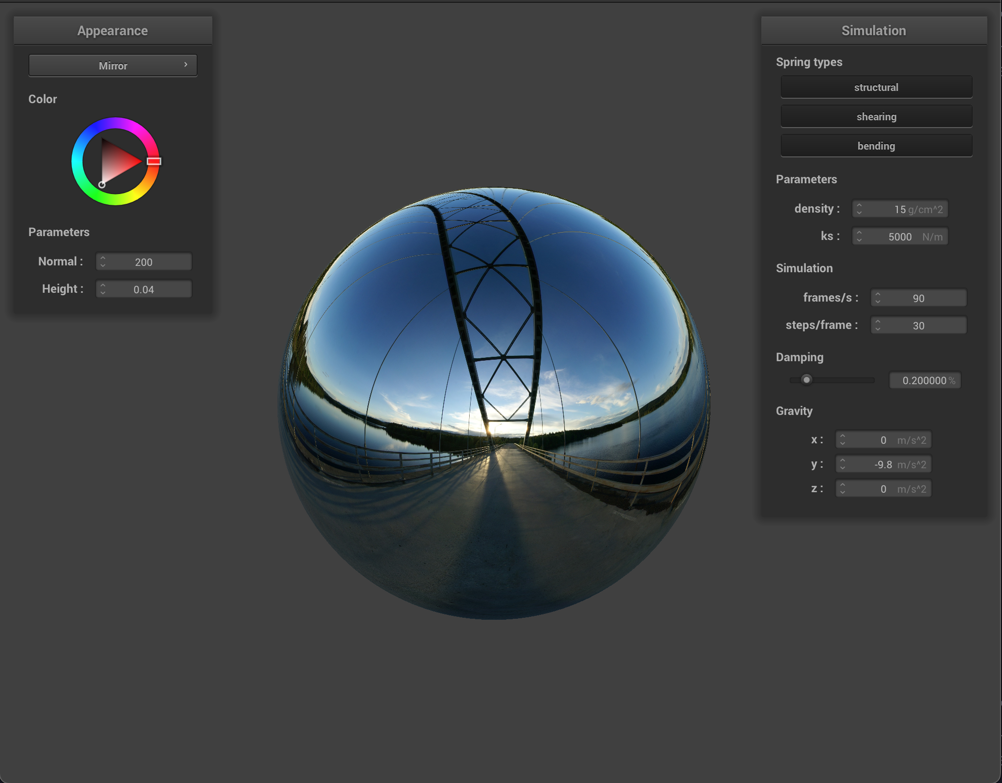
Mirror Shader
The mirror shader uses a cube map to get the color that is reflected on the surface from the environment. The ray is cast from the camera, and to get the incident ray, we first compute the projection vector of the camera ray \(r_c\) onto the vertex normal \(\vec{n}\) and add it scaled by a factor of 2 to our camera ray:\begin{equation*} w_o = 2\cdot \text{proj}_{r_{c}}(\vec{n}) + r_{c} \end{equation*} Then we can sample the cube map given the direction vector to get the color of the vertex.