Spatial Indexing

What are They?

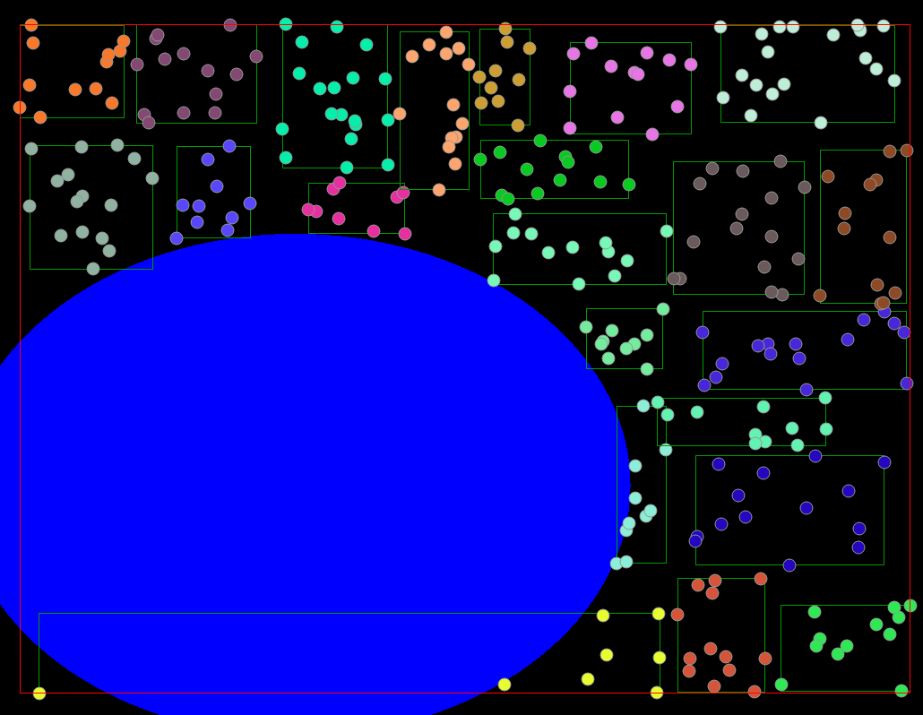
Indexing often describes methods of storing and organizing large amounts of data. In this case, spatial indexing is for the storage and querying of large amounts of spatial data, typically used in path planning and navigation. For example, map applications can store registered location data to provide the user with nearby attractions/restaurants they may want to visit.

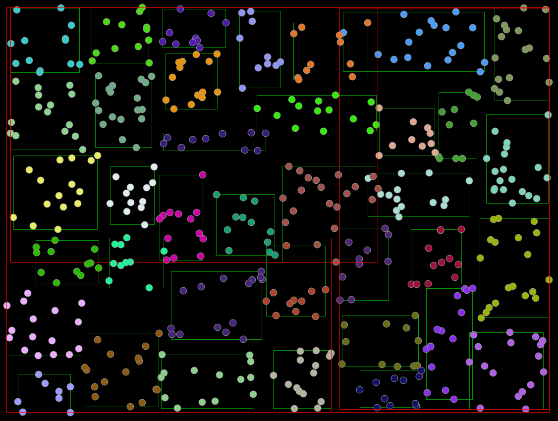
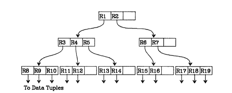
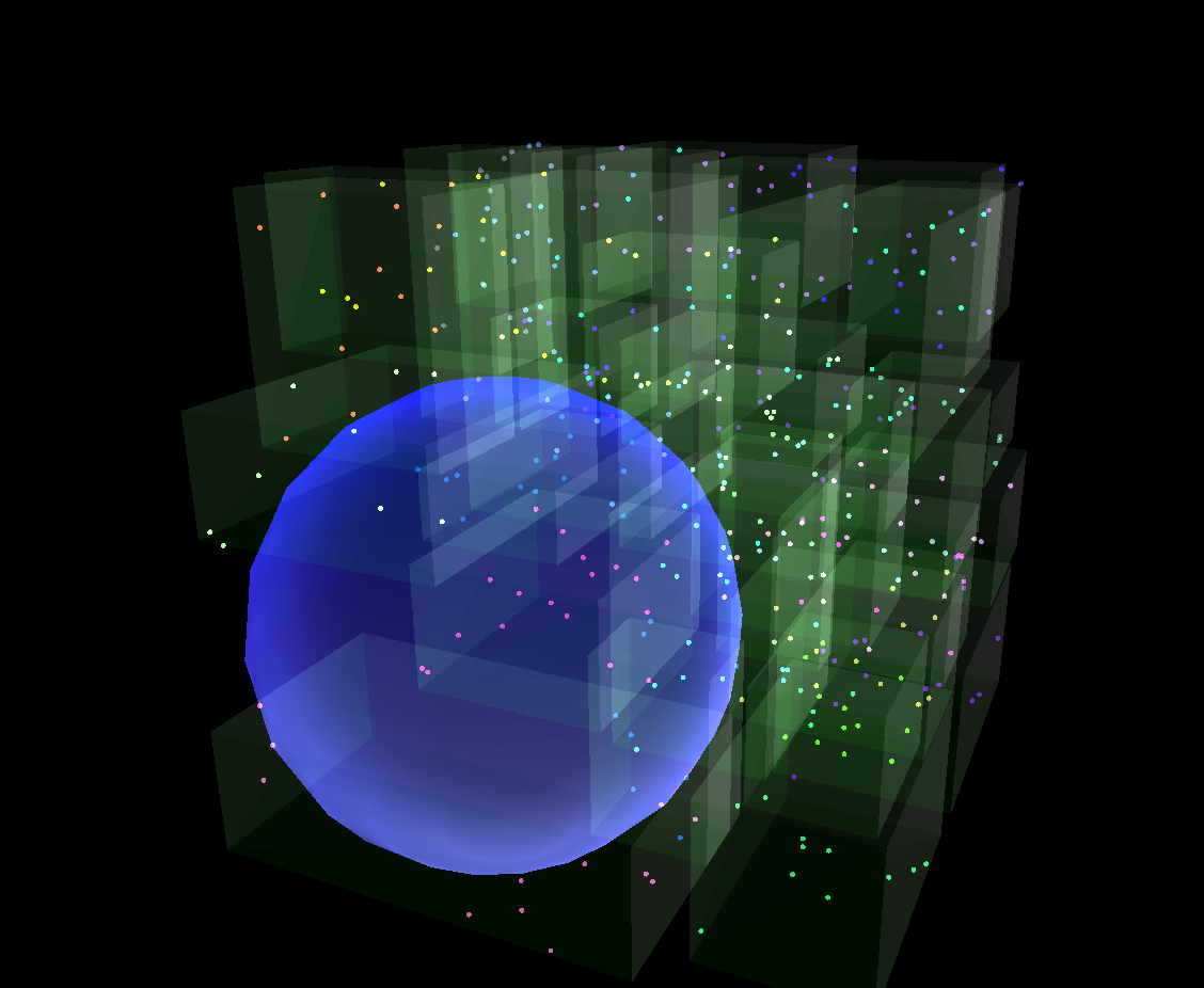
Spatial trees can be of different types, some are balanced trees (R-Trees) where they try to minimize tree depth. Others are adaptive and bound the number of children per tree node (Quad-trees, Octrees, ...).

R-Trees

For my project, I chose to implement an RTree compared to other spatial indexing methods such as K-D trees/Octrees for its ability to store not only points but higher-dimensional objects.

IndexRecords and IndexPointers

The tree stores objects called index records and index pointers, both of which are a type of rtree entry. This means they contain information on their bounding box. The only difference is that index pointers are stored in the non leaf nodes while index records are stored in the leaf nodes.

Each index record is of the form: \begin{equation*} (\text{id}, \text{bounding box}) \end{equation*} where id is the id of the item we want to store and the bounding box is an array of tuples: \begin{equation*} [(a_{1}, b_{1}), \ldots, (a_{n}, b_{n})] \end{equation*} where in the \(i\)-th dimension, the point location \(p_{i}\) on the object is such that:\begin{equation*} a_{i} \leq p_{i} \leq b_{i} \end{equation*}

An index pointer also has bounding box and also points to either a leaf node or a branch node

Leaf Nodes and Branch Nodes

These are the nodes that store the index records and index pointers of the tree. Leaf nodes store an array of index records while branch nodes store an array of index pointers.

The Insert Algorithm

In growing the tree, we want to ensure that there is as little bound overlap between bounds as possible between neighboring nodes. This way, searching for a node becomes easier if there is less bound overlap.

Choose Leaf

We first explore down the tree finding the best node to insert into at each level. This is determined by the ChooseLeaf function, which picks a leaf that results in the least bound expansion if we were to insert our index record.

Once we have found our leaf node, we insert the index record, and propagate the change upwards, updating the tree bounds of the leaf node, branch nodes, and index pointers that we traversed.

Splitting the Tree

If insertion into the leaf node results in the number of children exceeding a chosen max size, we split the node into two leaf nodes. The children are redistributed among the leaf nodes and again, changes are propagated upwards. This propagation can cause subsequent splits to happen.

If the root node splits, we create a new root and set the split nodes as the new root's children

Splitting the Node

Finding a good split is difficult to accomplish efficintly, as the new nodes must share as little bound overlap as possible. There are two methods of splits that provide similar results. These are the Linear and Quadratic splits, which involve picking two seeds/index record that we start off with in our split node. We then determine the subsequent index record allocation by some heuristic.

Search Algorithm

The search algorithm is what makes the R-Tree useful. The idea is to start with a small radius that we search around and continually grow this radius until we find the node we are looking for. In practice, we use a priority queue to store the index pointer/index record that is closest to the query. At each pop, we can either dump the contents of the index pointer into the priority queue or if we see an index record, that is the closest value to the query.

Delete Method

The delete method is similar to the search method, but we delete a node once it has been found and propagate any bound changes up. If a node is underfull, we remove the node from the tree. After the delete operation, we reinsert all of its children.

This means that the tree must be able to handle insertion of index pointers also. It is recommended that the minimum number of children is \(40\%\) of the max number of children of a tree node.

R*-Trees

R* Trees are very similar to R-Trees but considers two modifications. One problem with the R-Tree is once we insert, we are stuck with having to work around the bounds calculated from previous insertions. R* Trees solve this with an overflow method.

The second modification is in the splitting process. Rather than picking two seeds, we sort the objects along every dimension and choosing the split along the dimension that results in the least overlap.

There are also a couple smaller modifcations which try to ensure that the rectangular bounds of the tree nodes are as square as possible which results in a cleaner packing of bounds.

Overflow Treatment

If there are too many index records/index pointers in a leaf node/branch node after an insertion, we first attempt to reinsert all children back into the tree. This can cause some subsequent splitting, so we assert that this overflow can only happen once per level of the tree (prevent loops). If overflow has occurred, we do the usual tree split and propagation upwards.

Conclusion

R*-Trees although not optimal in terms of keeping bound overlap minimal is known for being efficient enough in practice. If the distribution of the data is known before hand, there are methods to construct an R*-Tree through sorting and loading the data all in at once.