Surface Reconstruction

Implicit and Explicit Reconstruction

In surface reconstruction, we attempt to recover a mesh that describes the surface from a point cloud. Reconstruction can be divided between two types, one is implicit and the other explicit.

In explicit reconstruction, we construct the mesh through the physical properties of the mesh, for example, one method involves rolling a ball over the point cloud to define the surface. The crust method involves defining a Delaunay triangulation based on the spatial properties of the points.

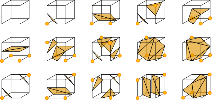
Implicit reconstruction on the other hand defines an implicit function over the 3d space. Through this, we can determine if a point in lies inside or outside of the mesh. A mesh generating algorithm such as marching cubes is then used to construct the triangles.

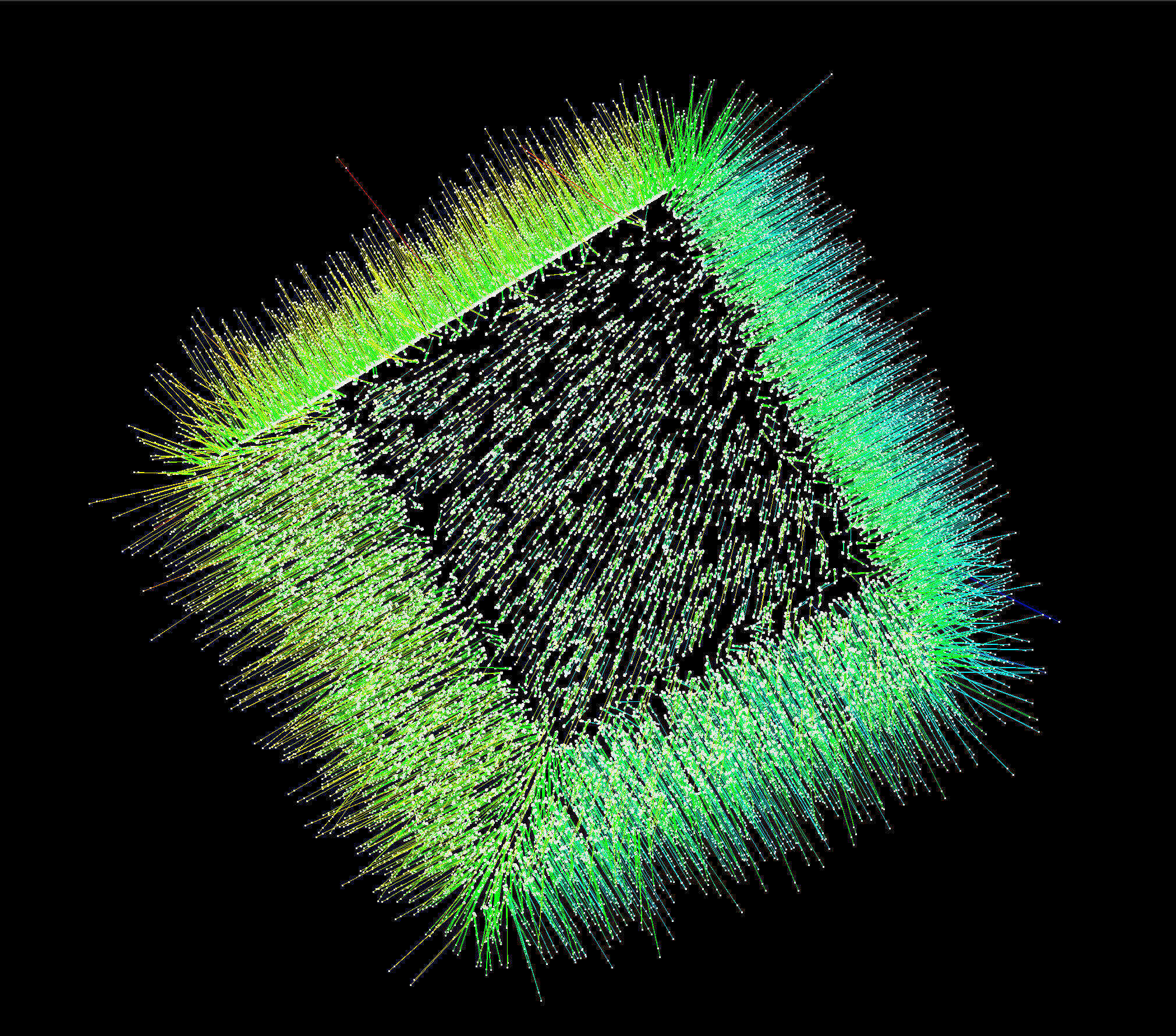
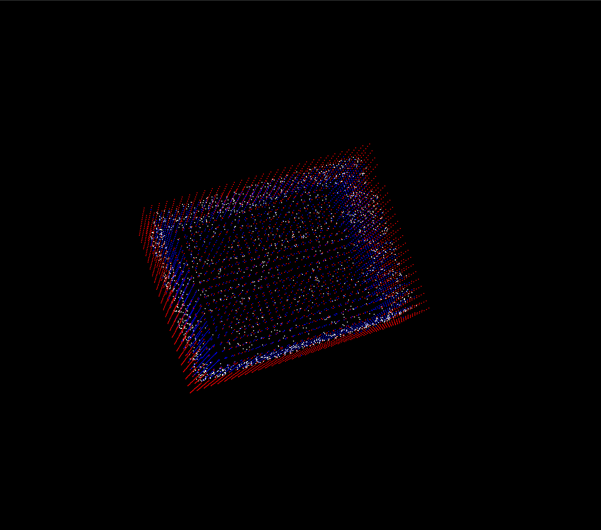
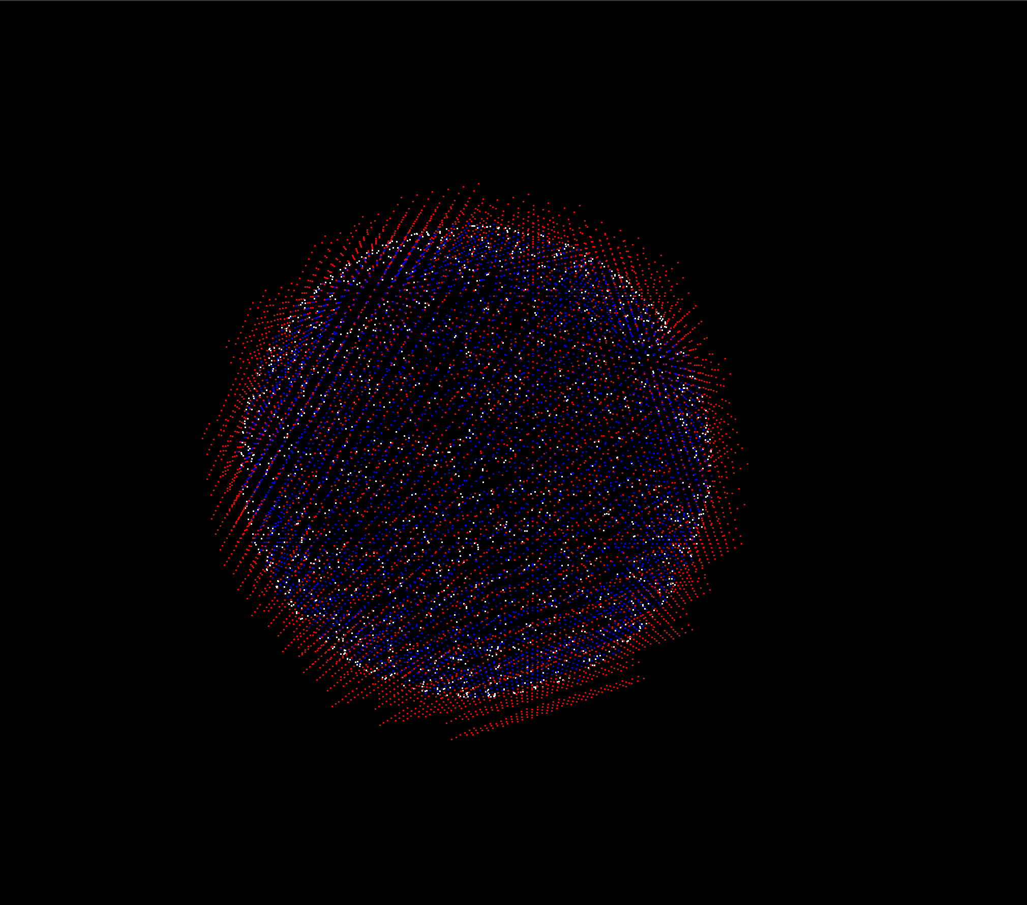
In reconstruction, the aim is to build a watertight mesh that is robust to noise. Noise in this case are the inaccuracies in the point cloud that we are given arising from sampling error.

Hoppe's Algorithm

Hoppe's research paper proposes a method of obtaining the surface normals of an object, and later proposes a signed distance function that can be used to estimate the triangles computed during marching cubes.

Normal Approximation

To retrieve the normals, we utilize PCA (Principal Component Analysis) on a patch of points. This gives us vectors describing the orientation of the patch, and subsequently the vector of smallest magnitude is the normal to the surface:

The smallest vector can either be pointing towards the inside of the object or outside, so to fix the traversal, we construct a Riemannian Graph (all vertices connected to their 15 closest neighbors) and decorate it with a Euclidean MST to ensure we can traverse all vertices. The traversal order is then decided by the mst with the weight function: \begin{equation*} w(u, v) = 1 - \lvert u.N \cdot v.N \rvert \end{equation*} which is the dot product between their normals. This is because if we consider two points very close to each other on a mesh surface, their normals will approximately be parallel. Therefore, the given weight function assigns a small weight to edges that join parallel normals.

This image shows the input normals, with incorrectly oriented normals in red. The traversal order is established which is the blue line, and in the zoom-in, the vertex after the blue line has its normal flipped because its orientation is incorrect wrt to the previous normal.

To begin traversal, we choose the point with the largest \(x\) component as our start vertex, ensure its normal is facing in the same direction as \(\begin{bmatrix} 1 \\ 0 \\ 0 \end{bmatrix}\):\begin{equation*} \vec{v} \cdot \begin{bmatrix} 1 \\ 0 \\ 0 \end{bmatrix} > 0 \end{equation*} and if not, we take \(\vec{v} \cdot -1\). We then traverse the mst with our normal orienting method until every normal points away from the interior of the mesh.

Signed Distance Function

A signed distance function \(f(p)\) gives us two pieces of information:

• A point is inside the mesh if \(f(p) < 0\), outside the mesh if \(f(p) > 0\), and on the mesh if \(f(p) = 0\).
• \(\lvert f(p) \rvert\) gives us the distance a point is the the surface.

Evaluating the sdf for our mesh at point \(p\) is then done by choosing a point from our sample, \(s\), that is closest to \(p\)and obtaining the distance from \(p\) to the tangent plane,\(s.TP\)of \(s\). We multiply the result by:\begin{equation*} \text{sign}\{\text{proj}_{s.TP}(p) \cdot s.N\} \end{equation*}(\(+1\) if the point is outside, \(-1\) if inside, \(0\) otherwise.)

Marching Cubes

The marching cubes algorithm is based on using a lookup table to determine the mesh triangles of a given finite element, in this case, we discretize the space into cubic subdivisions. We then use our signed distance function to determine the triangles that the given finite element has.

We intersect our cube with our mesh and evaluate the sdf on the cube's vertices. We mark the vertices that are inside the mesh as orange and we match them with the triangles found in the image above. After running this on all cubes that intersect our mesh, we obtain the final mesh.

Poisson Reconstruction

Solving the Matrix